Assignment 1

Problem 1:
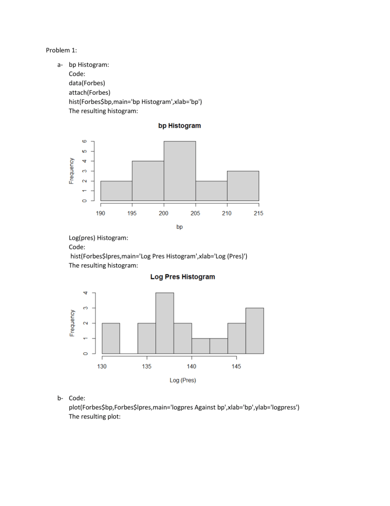
a- bp Histogram:
Code:
data(Forbes)
attach(Forbes)
hist(Forbes$bp,main='bp Histogram',xlab='bp')
The resulting histogram:
Log(pres) Histogram:
Code:
hist(Forbes$lpres,main='Log Pres Histogram',xlab='Log (Pres)')
The resulting histogram:
b- Code:
plot(Forbes$bp,Forbes$lpres,main='logpres Against bp',xlab='bp',ylab='logpress')
The resulting plot:
c- Code used:
model <- lm(Forbes$lpres ~ Forbes$bp, data = Forbes)
model
Result:
B0 = -42.14 / B1 = 0.8955
log (press) = -42.14 + 0.8955bp + error
d- Derived Line:
Code:
abline(lm(lpres ~ bp, data = Forbes), col = "blue")
Result plot:
e- For bp = 207, lpres ~ -42.14 + 0.8955 x 207 = 143.23
f- Code:
residual <- resid(model)
plot(fitted(model), residual)
abline(0,0)
Resulting Plot:
g- From part a, we notice which boiling points and pressures are recorded with highest
frequencies. Regarding the boiling points, there is one peak, and the recorded boiling point with
highest frequency is 200 – 205 F. Regarding the log (pres), the one with highest frequency is
between 135 and 140. From part b, we notice a positive relation between boiling point and
log(pres); as boiling point increases, log (pres) increases. From part c, we notice that the slope
(B1) is positive (which is expected from the observation in part b). We also notice that the
intercept is low and negative. This shows that at low boiling points, log(pres) is low. From part d,
we notice that points that are outside the regression line are little. This shows that the mode is
accepted. Part e is a calculation from the regression model used. From part e, we notice that the
spread of residuals is acceptable and the model does not need change.
Problem 2:
1- Predictor: ppgdp function
Response: fertility
2- After importing the Excel file UN11 into R, the following code was used:
library(alr3)
data(UN11)
plot(UN11$ppgdp,UN11$fertility,main='Scatterplot',xlab='ppgdp',ylab='Fertility')
The resulting scatterplot is as follows:
The above scatterplot shows that the fertility indicator varies from 1 to 7 at a common range of
ppgdp. The variance is not constant and the correlation is not linear. Hence, we say that a
straight-line mean function is not plausible in such case for a summary of the graph.
3-
Used Code:
plot(log(UN11$ppgdp),log(UN11$fertility),main='Log Scatterplot',xlab='Log ppgdp',ylab='Log
Fertility')
Since the natural logarithm is needed, the base is set to default.
Resulting scatter plot:
The simple linear regression seems plausible for summary for the graph (using log scale) since
the variance is almost constant.
Problem 3:
1- Computation of the mean and variance using R:
Codes:
data(wblake)
attach(wblake)
meanLength <- with(wblake, tapply(Length, Age, mean))
print(meanLength)
varLength <- with(wblake, tapply(Length, Age, var))
print(varLength)
The resulting mean values are as follows:
The resulting variance values are as follows:
2- Average Length vs. Age Groups
AgeGroup <- sort(unique(wblake$Age))
plot(AgeGroup,meanLength,main='Average Length vs. Age Groups',xlab='Age
Group',ylab='Average Length')
Code to plot the graph showing all the recorded lengths with average line:
plot(wblake$Age,wblake$Length,main='Length vs. Age Groups with Average Line',xlab='Age
Group',ylab='Length')
lines(AgeGroup,tapply(wblake$Length,wblake$Age,mean))
Resulting Graph:
Comparison with Figure 1.5:
This graph is the same of Figure 1.5 except that Figure 1.5 is drawn at another scale and that it shows
linear regression of the data.
3- Standard Deviation vs. Age:
Code:
stdLength <- with(wblake, tapply(Length, Age, sd))
plot(AgeGroup,stdLength,main='Std Length vs. Age Groups',xlab='Age Group',ylab='STD Length')
The plot shows difference in the standard deviation depending on age groups. The plot is not a
null plot. Hence, the variance function is not constant.
Problem 4:
Code used:
data(water)
attach(water)
pairs(Year~BSAAM+APMAM+APSAB+APSLAKE+OPBPC+OPRC+OPSLAKE)
Resulting Plot:
From these scatterplot matrix, it seems that year would not be used for the prediction because the
scatter plots do not show steady relations between change in years and water supply.
Other insights from the matrix:
The relation between BSAAM and (OPBC, OPRC and OPSLAKE) is stronger than the relation between
BSAAM and (APMAM, APSAB and APSLAKE). The relation between the locations starting with the A with
each other is stronger than their relations with those starting with the O. Similarly, the relation between
the locations starting with the O with each other is stronger than their relation with those starting with
the A. Conclusion: BSAAM could be an indicator to predict the runoff for those starting with the O. And
knowing the runoffs in one of those starting with A could be an indicator for the others starting with the
A. Finally, knowing the runoffs in one of those starting with O could be an indicator for the others
starting with the O.
Problem 5:
Example 1: X is uniformly distributed on interval [-1, 1]. Y = |X|. In this case, if X<0, Y = -X and if X>0, Y =
X. These two RVs are dependent, where Y depends on X. Let’s check for correlation:
Check if Cov [X, Y] = 0: Cov [X, Y] = E [XY] – E[X] x E[Y]
1
E[X] = ∫−1 𝑥𝑑𝑥 =
1
2
1
− 2 = 0 => E[X] x E[Y] = 0
XY = -𝑋 2 𝑖𝑓 𝑋 < 0 𝑎𝑛𝑑 𝑋𝑌 = 𝑋 2 𝑖𝑓 𝑋 > 0
0
1
E [XY] = E[XY| X<0] + E[XY| X>0] = ∫−1 −𝑋 2 𝑑𝑥 + ∫0 𝑋 2 𝑑𝑥 = -1\3 + 1/3 = 0
Therefore Cov [X, Y] = E [XY] – E[X] x E[Y] = 0 – 0 = 0. Hence X and Y are independent but uncorrelated.
Example 2: X is a discrete RV that takes three values: -1, 0 and 1 with P(X=-1) = P(X=0) = P(X=1) = 1/3
And Y = 1 if X = 0, and Y = 0 otherwise. The values of Y depend on X. Let’s check for correlation:
Check if Cov [X, Y] = 0: Cov [X, Y] = E [XY] – E[X] x E[Y]
E[X] = -1 x P (X=-1) + 0 x P (X=0) + 1 x P (X=1) = -1/3 + 0 + 1/3 = 0. Hence, E[X] x E[Y] = 0.
E[XY] = E[XY|X=-1] + E[XY|X=0] + E[XY|X=1]. If X=1 or X=-1, Y = 0. Hence, XY = 0. If X=1, Y = 1 and XY = 0.
Hence, E[XY] = 0 + 0 + 0 = 0
Problem 6:
Formula to Prove: Var [Y] = E [Var [Y|X]] + Var [E [Y|X]]
E [Var [Y|X]] = E {E [𝑌 2 |𝑋] - E [Y|X]2 } = E {E [𝑌 2 |𝑋] - f(x)2 } = E [𝑌 2 ] – E [f(x)2 ]
Var [E [Y|X]] = E [f(x)2 ] – E [[f(x)]]2 = E [f(x)2 ] – (E [Y])2
Therefore, E [Var [Y|X]] + Var [E [Y|X]] = E [𝑌 2 ] – E [f(x)2 ] + E [f(x)2 ] – (E [Y])2 = E [𝑌 2 ] - (E [Y])2 = Var [Y]
Problem 7:
Case 1: E [e] = 0
E [𝑒 2 ] = 𝑉𝑎𝑟 [𝑒] = 𝐸[𝑉𝑎𝑟[𝑒|𝑋]] + 𝑉𝑎𝑟 [𝐸 [𝑒|𝑥]]
𝐸[𝑉𝑎𝑟[𝑒|𝑋]] = 𝜎 2 and 𝑉𝑎𝑟 [𝐸 [𝑒|𝑥]] >= 0
Therefore, E [𝑒 2 ] ≥ 𝜎 2
Case 2: E [e] = c ≠0
E [𝑒 2 ] = 𝑉𝑎𝑟 [𝑒] + [E [e] ]2 = 𝐸[𝑉𝑎𝑟[𝑒|𝑋]] + 𝑉𝑎𝑟 [𝐸 [𝑒|𝑥]] + [E [e] ]2 = 𝜎 2 +𝑉𝑎𝑟 [𝐸 [𝑒|𝑥]] + [E [e] ]2
And in case [E [e] ]2 > 0 and 𝑉𝑎𝑟 [𝐸 [𝑒|𝑥]] >= 0. Therefore, in this case E [𝑒 2 ] > 𝜎 2
In this case, since [E [e] ]2 > 0, E [𝑒 2 ] > 𝜎 2 . In order to generalize E [𝑒 2 ] = 𝜎 2 , we would have E[e] = 0. Or
else, if [E [e] ]2 > 0, E[𝑒 2 ] is calculated as higher than 𝜎 2 .