Learning Semantic Boundaries from Noisy Annotations

Devil is in the Edges: Learning Semantic Boundaries from Noisy Annotations
David Acuna1,2,3
1
NVIDIA
{davidj,
Amlan Kar2,3
Sanja Fidler1,2,3
2
3
University of Toronto
Vector Institute
amlan}@cs.toronto.edu, [email protected]
STEAL: Semantic Thinning Edge Alignment Learning
arXiv:1904.07934v2 [cs.CV] 9 Jun 2019
Abstract
Devil is in the Edges
We tackle the problem of semantic boundary prediction,
which aims to identify pixels that belong to object(class)
boundaries. We notice that relevant datasets consist of a
significant level of label noise, reflecting the fact that precise annotations are laborious to get and thus annotators
trade-off quality with efficiency. We aim to learn sharp and
precise semantic boundaries by explicitly reasoning about
annotation noise during training. We propose a simple new
layer and loss that can be used with existing learning-based
boundary detectors. Our layer/loss enforces the detector to
predict a maximum response along the normal direction at
an edge, while also regularizing its direction. We further
reason about true object boundaries during training using
a level set formulation, which allows the network to learn
from misaligned labels in an end-to-end fashion. Experiments show that we improve over the CASENet [36] backbone network by more than 4% in terms of MF(ODS) and
18.61% in terms of AP, outperforming all current state-ofthe-art methods including those that deal with alignment.
Furthermore, we show that our learned network can be used
to significantly improve coarse segmentation labels, lending
itself as an efficient way to label new data.
labeled ground-truth
active alignment
labeled ground-truth
coarse-to-fine segmentation
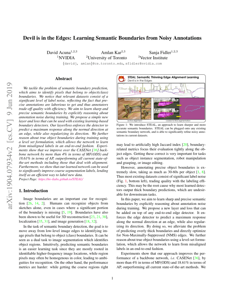
Figure 1: We introduce STEAL, an approach to learn sharper and more
accurate semantic boundaries. STEAL can be plugged onto any existing
semantic boundary network, and is able to significantly refine noisy annotations in current datasets.
may lead to artificially high Jaccard index [20], boundaryrelated metrics focus their evaluation tightly along the object edges. Getting these correct is very important for tasks
such as object instance segmentation, robot manipulation
and grasping, or image editing.
However, annotating precise object boundaries is extremely slow, taking as much as 30-60s per object [1, 8].
Thus most existing datasets consist of significant label noise
(Fig. 1, bottom left), trading quality with the labeling efficiency. This may be the root cause why most learned detectors output thick boundary predictions, which are undesirable for downstream tasks.
In this paper, we aim to learn sharp and precise semantic
boundaries by explicitly reasoning about annotation noise
during training. We propose a new layer and loss that can
be added on top of any end-to-end edge detector. It enforces the edge detector to predict a maximum response
along the normal direction at an edge, while also regularizing its direction. By doing so, we alleviate the problem
of predicting overly thick boundaries and directly optimize
for Non-Maximally-Suppressed (NMS) edges. We further
reason about true object boundaries using a level-set formulation, which allows the network to learn from misaligned
labels in an end-to-end fashion.
Experiments show that our approach improves the performance of a backbone network, i.e. CASENet [36], by
more than 4% in terms of MF(ODS) and 18.61% in terms of
AP, outperforming all current state-of-the-art methods. We
Project Page: https://nv-tlabs.github.io/STEAL/
1. Introduction
Image boundaries are an important cue for recognition [26, 14, 2]. Humans can recognize objects from
sketches alone, even in cases where a significant portion
of the boundary is missing [5, 19]. Boundaries have also
been shown to be useful for 3D reconstruction [23, 21, 38],
localization [35, 31], and image generation [18, 32].
In the task of semantic boundary detection, the goal is to
move away from low-level image edges to identifying image pixels that belong to object (class) boundaries. It can be
seen as a dual task to image segmentation which identifies
object regions. Intuitively, predicting semantic boundaries
is an easier learning task since they are mostly rooted in
identifiable higher-frequency image locations, while region
pixels may often be homogenous in color, leading to ambiguities for recognition. On the other hand, the performance
metrics are harder: while getting the coarse regions right
1
further show that our predicted boundaries are significantly
better than those obtained from the latest DeepLab-v3 [9]
segmentation outputs, while using a much more lightweight
architecture. Our learned network is also able to improve
coarsely annotated segmentation masks with 16px, 32px error improving their accuracy by more than 20% IoU and
30% IoU, respectively. This lends our method as an efficient means to collect new labeled data, allowing annotators
to coarsely outline objects with just a few clicks, and generating finer ground-truth using our approach. We showcase
this idea by refining the Cityscapes-coarse labelset, and exploiting these labels to train a state-of-the-art segmentation
network [9]. We observe a significant improvement of more
than 1.2% in some of the refined categories.
2. Related Work
Semantic Boundary Detection. Learning-based semantic edge detection dates back to [28] which learned a classifier that operates on top of a standard edge detector. In [15],
the authors introduced the Semantic Boundaries Dataset
(SBD) and formally studied the problem of semantic contour detection in real world images. They proposed the idea
of an inverse detector which combined bottom-up edges and
top-down detection. More recently, [36] extended the CNNbased class-agnostic edge detector proposed in [34], and allowed each edge pixel to be associated with more than one
class. The proposed CASENet architecture combined low
and high-level features with a multi-label loss function to
supervise the fused activations.
Most works use non-maximum-suppression [6] as a
postprocessing step in order to deal with the thickness of
predicted boundaries. In our work, we directly optimize for
NMS during training. We further reason about misaligned
ground-truth annotations with real object boundaries, which
is typically not done in prior work. Note that our focus here
is not to propose a novel edge-detection approach, but rather
to have a simple add-on to existing architectures.
The work most closely related to ours is SEAL [37], in
that it deals with misaligned labels during training. Similar
to us, SEAL treats the underlying ground truth boundaries
as a latent variable that is jointly optimized during training.
Optimization is formulated as a computationally expensive
bipartite graph min-cost assignment problem. In order to
make optimization tractable, there are no pair-wise costs,
i.e. two neighboring ground-truth pixels can be matched to
two pixels far apart in the latent ground-truth, potentially
leading to ambiguities in training. In our work, we infer
true object boundaries via a level set formulation which preserves connectivity and proximity, and ensures that the inferred ground-truth boundaries are well behaved. Moreover,
SEAL is limited to the domain of boundary detection and
needs to have reasonably well annotated data, since alignment is defined as a one-to-one mapping between annotated
and inferred ground-truth. In our method, substantial differences (topology and deviation) in ground truth can be
handled. Our approach can thus be naturally used to refine
coarse segmentation labels, lending itself as a novel way to
efficiently annotate datasets.
Level Set Segmentation. Level Set Methods [27] have
been widely used for image segmentation [7, 12, 30, 17,
24, 4, 22, 13] due to their ability to automatically handle
various topological changes such as splitting and merging.
Most older work derived different level set formulations
on top of standard image gradient observations, while recent work swapped those with neural network outputs [17].
In [24], the authors proposed a deep structured active contours method that learns the parameters of an active contour
model using a CNN. [20] introduced a method for object
proposal generation, by learning to efficiently place seeds
such that critical level sets originating from these seeds hit
object boundaries. In parallel work, [33] learns CNN feature extraction and levelset evolution in an end-to-end fashion for object instance annotation. In our work, we exploit
level set optimization during training as a means to iteratively refine ground-truth semantic boundaries.
3. The STEAL Approach
In this section, we introduce our Semantically Thinned
Edge Alignment Learning (STEAL) approach. Our method
consists of a new boundary thinning layer together with a
loss function that aims to produce thin and precise semantic edges. We also propose a framework that jointly learns
object edges while learning to align noisy human-annotated
edges with the true boundaries during training. We refer to
the latter as active alignment. Intuitively, by using the true
boundary signal to train the boundary network, we expect
it to learn and produce more accurate predictions. STEAL
is agnostic to the backbone CNN architecture, and can be
plugged on top of any existing learning-based boundary detection network. We illustrate the framework in Fig. 2.
Subsec. 3.1 gives an overview of semantic boundary detection and the relevant notation. Our boundary thinning
layer and loss are introduced in Subsec. 3.3. In Subsec. 3.4,
we describe our active alignment framework.
3.1. Semantic Aware Edge-Detection
Semantic Aware Edge-Detection [36, 37] can be defined
as the task of predicting boundary maps for K object classes
given an input image x. Let ykm ∈ {0, 1} indicate whether
pixel m belongs to class k. We aim to compute the probability map P (yk |x; θ), which is typically assumed to decompose into a set of pixel-wise probabilities P (ykm |x; θ)
modeled by Bernoulli distributions. It is computed with a
convolutional neural network f with k sigmoid outputs, and
parameters θ. Each pixel is thus allowed to belong to multiple classes, dealing with the cases of multi-class occlusion
fixed convolution
(normal estimation)
normal angles
fixed convolution
(normal estimation)
✓
boundary
classification layer
direction
loss
boundary
classif. loss
NMS loss
softmax
boundary detection
network
refined
labels
annotated
ground-truth
active
alignment
NMS architecture
training
inference
Figure 2: STEAL architecture. Our architecture plugs on top of any backbone architecture. The boundary thinning layer acts upon boundary classification
predictions by computing the edge normals, and sampling 5 locations along the normal at each boundary pixel. We perform softmax across these locations,
helping us enhance the boundary pixels as in standard NMS. During training, we iteratively refine ground-truth labels using our predictions via an active
alignment scheme. NMS and normal direction losses are applied only on the (refined) ground-truth boundary locations.
boundaries. Note that the standard class-agnostic edge detection can be seen as a special case with k = 1 (consuming
all foreground classes).
Semantic Edge Learning. State-of-the-art boundary detectors are typically trained using the standard binary cross
entropy loss adopted from HED [34]. To deal with the high
imbalance between the edge and non-edge pixels, a weighting term β = |Y − |/|Y | is often used, where |Y − | accounts
for the number of non-edge pixels among all classes in the
mini-batch, and |Y | is the total number of pixels. In the
multi-class scenario, the classes are assumed to be independent [36, 37]. Therefore, in learning the following weighted
binary cross-entropy loss is minimized:
X
LBCE (θ) = −
log P (yk |x; θ)
k
=−
XX
k
{β ykm log fk (m|x, θ)+
(1)
m
+ (1 − β)(1 − ykm ) log(1 − fk (m|x, θ))}
where y indicates the ground-truth boundary labels.
3.2. Semantic Boundary Thinning Layer
In the standard formulation, nearby pixels in each boundary map are considered to be independent, and can cause the
predictions to “fire” densely around object boundaries. We
aim to encourage predictions along each boundary pixel’s
normal to give the maximal response on the actual boundary. This is inspired by edge-based non-maximum suppression (NMS) dating back to Canny’s work [6]. Furthermore,
we add an additional loss term that encourages the normals
estimated from the predicted boundary maps to agree with
the normals computed from ground-truth edges. The two
losses work together in producing sharper predictions along
both the normal and tangent directions.
3.3. Thinning Layer and NMS Loss
Formally, during training we add a new deterministic
layer on top of the boundary prediction map. For each posi-
tive ground-truth boundary pixel p for class k we normalize
the responses along the normal direction d~kp as follows:
hk (p|x, θ) = PL
exp(fk (p|x, θ)/τ )
t=−L
where:
exp(fk (pt |x, θ)/τ )
x(pt ) = x(p) + t · cos d~p
y(pt ) = y(p) + t · sin d~p
(2)
(3)
(4)
Here, t ∈ {−L, −L + 1, . . . , L}, and L denotes the maximum distance of a pixel pt from p along the normal. See
Fig. 2 for a visualization. We compute the normal direction d~kp from the ground-truth boundary map using basic
trigonometry and a fixed convolutional layer that estimates
second derivatives. The parameter τ in Eq. (2) denotes the
temperature of the softmax. We use L = 2 and τ = 0.1.
Intuitively, we want to encourage the true boundary pixel
p to achieve the highest response along its normal direction.
We do this via an additional loss, referred to as the NMS
loss, that pushes the predicted categorical distribution computed with h towards a Dirac delta target distribution:
XX
Lnms (θ) = −
log hk (p|x, θ)
(5)
k
p
Note that p indexes only the positive boundary pixels for
each class, other pixels do not incur the NMS loss. We compute fk (pt |x, θ) in Eq. (2) for non-integral locations using
a bilinear kernel.
Direction Loss. Ideally, the predicted boundaries would
have normal directions similar to those computed from the
ground-truth boundaries. We follow [3] to define the error
as the mean squared loss function in the angular domain:
XX
Ldir (θ) =
|| cos−1 hd~p , e~p (θ)i||,
(6)
k
p
with d~p the ground-truth normal direction in boundary pixel
p, and e~p the normal computed from the predicted boundary
map. We use the same convolutional layer on top of fk to
get ~e. Finally, we compute our full augmented loss as the
combination of the following three terms:
L = α1 LBCE + α2 Lnms + α3 Ldir
(7)
where α1 , α2 , α3 are hyper-parameters that control the importance of each term (see Experiments).
3.4. Active Alignment
Learning good boundary detectors requires high quality
annotated data. However, accurate boundaries are time consuming to annotate. Thus datasets tradeoff between quality
and annotation efficiency. Like [37], we notice that the standard SBD benchmark [15] contains significant label noise.
In this section, we propose a framework that allows us to
jointly reason about true semantic boundaries and train a
network to predict them. We adopt a level set formulation
which ensures that the inferred “true” boundaries remain
connected, and are generally well behaved.
Let ŷ = {ŷ1 , ŷ2 , ..., ŷK } denote a more accurate version
of the ground-truth label y, which we aim to infer as part of
our training procedure. We define ŷi as a curve. Our goal is
to jointly optimize for the latent variable ŷ and parameters
θ of the boundary detection network. The optimization is
defined as a minimization of the following loss:
X
log P (yk , ŷk |x; θ)
(8)
min L(ŷ, θ) = −
ŷ,θ
=−
∂φ
= gk (κ + c)|∇φ| + ∇gk · ∇φ
(12)
∂t
where c can be seen as a constant velocity that helps to avoid
certain local minima [7]. Eq. 12 can also be interpreted as
the Geodesic Active Contour formulation of the Level Set
Method [7, 27].
3.5. Learning
Minimizing Eq. (8) can be performed with an iterative
two step optimization process. In one step, we evolve the
provided boundary yk towards areas where the network is
highly confident. The number of evolution steps indexed by
t can be treated as a latent variable and ŷk is selected by
choosing the ŷkt that minimizes Eq. (8). In the second step,
we optimize θ using the computed yk .
Formally, we want to solve:
min L(ŷ, θ) = min min L(ŷ, θ)
θ
ŷ,θ
ŷ
(13)
where we iterate between holding θ fixed and optimizing ŷ:
k
X
Eq (11) follows the level-set approach [27], where the
curve ŷkt is a 0 level-set of an embedding function φ, i.e.
a set of points satisfying φ(.) = 0. By differentiating the
latter equation, it is easy to show that if ŷk evolves accord∂ ŷt
ing to ∂tk = β~n then the embedding function φ can be
~
deformed as ∂φ
∂t = β |∇φ| [7]. We can thus rewrite the evolution of ŷk in terms of φ as follows:
log P (yk |ŷk ) + log P (ŷk |x; θ)
min L(ŷk , θ) = min{− log P (ŷkt |x; θ) − C}
ŷk
k
The second term is the log-likelihood of the model and
can be defined as in the previous section. The first term
encodes the prior that encourages ŷk to be close to yk . Inspired by [7], we define this term with an energy that describes “well behaved” curves:
Z
gk (ŷk (q)) |ŷk0 (q)| ∂q
E(yk |ŷk , λ) =
(9)
q
where we define gk (.) as the following decreasing function:
λ
1
+√
(10)
gk = √
1 + yk
1 + fk
Here, λ is a hyper-parameter that controls the effect of yk .
Intuitively, this energy is minimized when the curve ŷk lies
in areas of high probability mass of fk , and is close, by a
factor of λ, to the given ground-truth yk .
We can minimize Eq. (9) via steepest-descent, where we
find the gradient descent direction that allows to deform the
initial ŷk0 (here we use the given noisy ground-truth as the
initial curve) towards a (local) minima of Eq. (9) [7]:
∂ ŷkt
= gk κ ~n − (∇gk · ~n)~n
(11)
∂t
Here κ is the Euclidean curvature and ~n is the inward normal to the boundary. Details of this computation can be
found in [7], Appendix B and C.
t
(14)
and optimizing θ via Eq. (7) while holding ŷ fixed. Here C
is a constant that does not affect optimization.
3.6. Coarse-to-Fine Annotation
Embedding the evolution of ŷ in that of φ has two main
benefits. Firstly, topological changes of ŷ are handled for
free and accuracy and stability can be achieved by using
proper numerical methods. Secondly, φ can be naturally
interpreted as a mask segmenting an object, where φ < 0
corresponds to the segmented region. Moreover, our approach can also be easily used to speed up object annotation. Assume a scenario where an annotator draws a coarse
mask inside an object of interest, by using only a few clicks.
This is how the coarse subset of the Cityscapes dataset has
been annotated [11]. We can use our learned model and
levelset formulation (Eq. (12)), setting λ = 0 and c = 1
to evolve the given coarse mask by t iterations to produce
an improved segmentation mask whose edges align with the
edges predicted by our model.
3.6.1
Implementation Details
Morphological Level Set. In this work, we follow a morphological approach to compute the differential operators
Metric
MF
(ODS)
AP
Method
CASENet
CASENet-S
SEAL
Ours (NMS Loss)
Ours (NMS Loss + AAlign)
CASENet
CASENet-S
SEAL
Ours (NMS Loss)
Ours (NMS Loss + AAlign)
aero
74.84
76.26
78.41
78.96
80.15
50.53
67.64
74.24
75.85
76.74
bike
60.17
62.88
66.32
66.20
67.80
44.88
53.10
57.45
59.65
60.94
bird
73.71
75.77
76.83
77.53
77.69
41.69
69.79
72.72
74.29
73.92
boat
47.68
51.66
52.18
54.76
54.26
28.92
40.51
42.52
43.68
43.13
bottle
66.69
66.73
67.52
69.42
69.54
42.97
62.52
65.39
65.65
66.48
bus
78.59
79.78
79.93
81.77
81.48
54.46
73.49
74.50
77.63
77.09
car
66.66
70.32
69.71
71.38
71.34
47.39
63.10
65.52
67.22
67.80
cat
76.23
78.90
79.37
78.28
78.97
58.28
75.26
77.93
76.63
77.50
chair
47.17
49.72
49.45
52.01
51.76
35.53
39.96
40.92
42.33
42.09
cow
69.35
69.55
72.52
74.10
73.61
45.61
60.74
65.76
70.67
70.05
table
36.23
39.84
41.38
42.79
42.82
25.22
30.43
33.36
31.23
32.11
dog
75.88
77.25
78.12
79.18
79.80
56.39
72.28
76.31
77.66
78.42
horse
72.45
74.29
74.57
76.57
76.44
48.45
65.15
68.85
74.59
74.77
mbike person plant sheep sofa train
tv
mean
61.78 73.10 43.01 71.23 48.82 71.87 54.93 63.52
65.39 75.35 47.85 72.03 51.39 73.13 57.35 65.77
65.98 76.47 49.98 72.78 52.10 74.05 58.16 66.79
66.71 77.71 49.70 74.99 50.54 75.50 59.32 67.87
67.68 78.16 50.43 75.06 50.99 75.31 59.66 68.15
42.79 55.38 27.31 48.69 39.88 45.05 34.77 43.71
56.57 70.80 33.91 61.92 45.09 67.87 48.93 57.95
58.31 73.76 38.87 66.31 46.93 69.40 51.40 61.02
61.04 77.44 38.28 69.53 40.84 71.69 50.39 62.32
61.28 77.52 39.02 68.51 41.46 71.62 51.04 62.57
Table 1: Comparison of our method in the re-annotated SBD test set vs state-of-the-art. Scores are measured by %.
Method
CASENet [36]
SEAL [37]
Ours
aero
83.3
84.9
85.8
bike
76.0
78.6
80.0
bird
80.7
84.6
85.6
boat
63.4
66.2
68.4
bottle
69.2
71.3
71.6
bus
81.3
83.0
85.7
car
74.9
76.5
78.1
cat
83.2
87.2
87.5
chair
54.3
57.6
59.1
cow
74.8
77.5
78.5
table
46.4
53.0
53.7
dog
80.3
83.5
84.8
horse
80.2
82.2
83.4
mbike
76.6
78.3
79.5
person
80.8
85.1
85.3
plant
53.3
58.7
60.2
sheep
77.2
78.9
79.6
sofa
50.1
53.1
53.7
train
75.9
77.7
80.3
tv
66.8
69.7
71.4
mean
71.4
74.4
75.6
Table 2: Results on SBD test following the original evaluation protocol, and test set from [15].
Metric
Method
CASENet
Ours (CASENet)
MF
Ours (CASENet)
(ODS)
+ NMS Layer
+ NMS Layer
+ Active Align
CASENet
Ours (CASENet)
AP
Ours (CASENet)
+ NMS Layer
+ NMS Layer
+ Active Align
Test NMS
X
X
X
X
X
X
Or. Test Set
62.21
63.20
64.84
64.15
65.93
64.83
42.99
34.60
44.83
53.67
60.10
57.98
Re-annot. Test Set
63.52
64.03
66.58
64.99
67.87
68.15
43.71
45.60
60.48
54.18
62.32
62.57
Table 3: Effect of the NMS Loss and Active Alignment on the SBD
dataset. Score (%) represents mean over all classes.
used in the curve’s evolution. This solution is based on numerical methods which are simple, fast and stable. Additionally, in this approach, the level set is just a binary piecewise constant function and constant reinitialization of the
level set function is not required. We refer the reader to [25]
for a more detailed explanation and implementation details.
Training Strategy. Our active alignment heavily relies on
the quality of the network’s predictions to iteratively refine
the noisy ground-truth. During initial stages of training, the
network is not confident and may lead us to infer potentially
noisier labels. We hence introduce alignment after the network’s accuracy starts to flatten. In our formulation, this can
be seen as setting λ = inf for a certain number of iterations.
In order to save on computation time, active alignment can
also be applied every n training iterations.
4. Experimental Results
In this section, we provide an extensive evaluation of our
approach on the standard SBD benchmark [15], as well as
on the Cityscapes dataset [11]. We further show how our
approach can be used to significantly improve coarse segmentation labels, mimicking a scenario where we train on
a labeled dataset with moderate noise, and use the trained
model to generate finer annotations from only coarsely annotated data (collected with less manual annotation effort).
Implementation Details. In all experiments, we select
CASENet [36] as the backbone network since it is the
current state-of-the-art semantic-aware-edge detection ar-
Metric
MF
(ODS)
AP
Method
Ours (CASENet)
Ours (CASENet)
+ NMS Layer
Ours (CASENet)
Ours (CASENet)
+ NMS Layer
Active Align
X
X
X
X
Noisy Train
64.03
64.10
68.15
45.60
45.41
62.57
Noisy Train ( +8px err)
50.58
52.69
56.41
29.32
27.60
43.97
Table 4: Effect of Active Alignment on the SBD dataset. Score (%)
represents mean over all classes.
chitecture. We re-implement CASENet in PyTorch following [36]. The performance of our reimplementation
(slightly better) is illustrated in tables as CASENet Ours
for fair comparison. We use 472 × 472 as the training
resolution. Training is done on an NVIDIA DGX Station using 4 GPUs with a total batch size of 8. We use
α1 = 1, α2 = 10, α3 = 1 in our loss function. For SBD,
we use a learning rate of 1e-7. At 20k iter, we decrease the
learning rate by a factor of 10 and set β = 0. Active alignment is done every 5k iter (λ = 1) starting at 55k iter. The
full model converges at about 70k iter and takes approximately two days to train. For Cityscapes, we set the learning
rate to be 5e-8, and decay is done every 20k iterations by a
factor of 20. Since images are more densely annotated, we
set the weights of the loss function to be 1. We do not use
active alignment in Cityscapes since the train set is finely
annotated. This is used later for the refinement of coarse
data. The model converges at around 60k iterations.
4.1. Datasets and Evaluation Metrics
Semantic Boundary Dataset (SBD) [15] contains 11355
images from the trainval set of PASCAL VOC2011, with
8498 images divided into training, and 2857 as test. This
dataset contains annotations following the 20-class definitions in PASCAL VOC. In our experiments, we randomly
select 100 images from the training set, which are used as
our inference. Training is performed on the remaining 8398
images and evaluation is done on test. We additionally report performance on the high-quality re-annotated SBD test
set from [37]. This constitutes 1059 images from SBD test.
Cityscapes Dataset [11] contains 5000 finely annotated
images divided into 2975 training, 500 inference, and 1525
test images. Since the boundaries are not provided and test
is held-out, we follow [36] to generate the ground truth
(a) Image
(b) CASENet
(c) Ours
(d) +Thinning Layer
(e) Ground-truth
Figure 3: Qualitative Results on the SBD Dataset.
Figure 4: Active Alignment. From Left-to-right (GT, Refined).
Metric
MF
(ODS)
AP
Method
Test NMS
CASENet
Ours(CASENet)
Ours(CASENet)
X
+ NMS LOSS
+ NMS LOSS
X
CASENet
Ours(CASENet)
Ours(CASENet)
X
+NMS LOSS
+NMS LOSS
X
road s.walk build. wall fence pole t-light t-sign veg terrain sky person rider
car truck bus train motor bike mean
87.06 75.95 75.74 46.87 47.74 73.23 72.70 75.65 80.42 57.77 86.69 81.02 67.93 89.10 45.92 68.05 49.63 54.21 73.74 68.92
87.23 76.08 75.73 47.86 47.57 73.67 71.77 75.19 80.58 58.39 86.78 81.00 68.18 89.31 48.99 67.82 50.84 55.30 74.16 69.29
88.13 76.53 76.75 48.70 48.60 74.21 74.54 76.38 81.32 58.98 87.26 81.90 69.05 90.27 50.93 68.41 52.11 56.23 75.66 70.31
88.08 77.62 77.08 50.02 49.62 75.48 74.01 76.66 81.51 59.41 87.24 81.90 69.87 89.50 52.15 67.80 53.60 55.93 75.17 70.67
88.94 78.21 77.75 50.59 50.39 75.54 76.31 77.45 82.28 60.19 87.99 82.48 70.18 90.40 53.31 68.50 53.39 56.99 76.14 71.42
54.58 65.44 67.75 37.97 39.93 57.28 64.65 69.38 71.27 50.28 73.99 72.56 59.92 66.84 35.91 56.04 41.19 46.88 63.54 57.65
68.38 69.61 70.28 40.00 39.26 61.74 62.74 73.02 72.77 50.91 80.72 76.06 60.49 79.43 40.86 62.27 42.87 48.84 64.42 61.30
88.83 73.94 76.86 42.06 41.75 69.81 74.50 76.98 79.67 56.48 87.73 83.21 68.10 91.20 44.17 66.69 44.77 52.04 75.65 68.13
89.54 75.72 74.95 42.72 41.53 65.86 67.55 75.84 77.85 52.72 82.70 79.89 62.59 91.07 45.26 67.73 47.08 50.91 70.78 66.44
90.86 78.94 77.36 43.01 42.33 71.13 75.57 77.60 81.60 56.98 87.30 83.21 66.79 91.59 45.33 66.64 46.25 52.07 74.41 68.89
Table 5: Results on the val set on the Cityscapes dataset. Training is done using the finely annotated train set. Scores are measured by %.
edges and use the inference images as our test set.
Evaluation Protocol: We follow the evaluation protocol
proposed in [37] which is considerable harder than the one
used in [15, 2, 36]. An important parameter is the matching
distance tolerance which is defined as the maximum slack
allowed for boundary predictions to be considered as correct matches to ground-truth. We follow [37] and set it
to be 0.0075 for SBD and 0.0035 for Cityscapes. For further comparisons, in Table 2 we also report the performance
with the original SBD evaluation protocol [15].
Coarse Label Simulation. In order to quantify the level
of annotation noise that our approach can handle, we synthetically coarsen the given labels following the procedure
described in [39]. This algorithm, inspired by the way that
coarse labels were collected in Cityscapes [11], erodes and
then simplifies the true labels producing controlled masks
with various qualities. In addition, we also compute the estimated number of clicks required to annotate such objects.
This is simulated by counting the number of vertices in the
simplified polygon.
Evaluation Metrics: We use two quantitative measures
to evaluate our approach in the task of boundary prediction.
1) We use maximum F-Measure (MF) at optimal dataset
scale (ODS), and 2) average precision (AP) for each class.
To evaluate the quality of the improved coarse segmentation
masks, we use the intersection-over-union (IoU) metric.
4.2. Semantic Boundary Prediction
Results and Comparisons. We first compare the performance of our approach vs current state-of-the-art methods.
Our baselines include CASENet [36], and the recently proposed CASENet-S and SEAL [37]. CASENet-S can be seen
as an improved version of CASENet, while SEAL builds on
top of CASENet-S and also deals with misaligned labels.
Table 1 illustrates per category performance in the high
quality re-annotated SBD test set. Surprisingly, by just introducing the NMS Layer on top of CASENet, our method
72
AVG MF (ODS)
70
Ours
DeepLab V3+
CASENet
Label Quality
Num.Clicks per Image
Test IoU
GrabCut
Ours(Coarse-to-Fine) IoU
68
66
64
62
60
0.001875
(~2.15px)
0.00375
(~4.30px)
Matching Threshold
0.00500
(~5.72px)
iou
Figure 5: Comparison of our boundaries vs those obtained from DeepLab
v3+’s segmentation masks. We perform 4.2% better at the strictest regime.
95
93
91
89
87
85
83
81
79
77
75
73
71
69
67
65
coarse
coarse-to-fine
4px error
70.34
91.22
68.74
92.78
8px error
44.76
78.95
70.32
88.16
16px error
26.78
62.20
69.76
82.89
32px error
14.64
41.31
62.82
76.20
Table 6: Refining coarse labels on SBD. Model is trained on the noisy
SBD training set (approx 4px error). The re-annotated test set is then simplified to simulate coarse data with a given quality (see main text). Score
(%) represents mean over all the 20 object classes.
Label Quality
Num.Clicks per Image
Test IoU
GrabCut
Ours(Coarse-to-Fine) IoU
4px error
175.23
74.85
26.00
78.93
8px error
95.63
53.32
28.51
69.21
16px error
49.21
33.71
29.35
58.96
32px error
27.00
19.44
25.99
50.35
Real Coarse
98.78
48.67
32.11
67.43
Table 7: Refining coarse labels on Cityscapes. Model trained on fine
Cityscapes trainset and used to refine coarse data. Real Coarse corresponds
to coarsely human annotated val set, while x-px error correspond to simulated coarse data. Score (%) represents mean over all 8 object classes.
ped rider car truck bus train mbike bike rest mIoU
category
Figure 6: Semantic Segmentation on Cityscapes val: Performance of
DeepLab V3+ when trained with fine data and (blue) vanilla train extra
set, (orange) our refined data (8 object classes) from train extra. We see
improvement of more than 1.2 IoU % in rider, truck and bus.
outperforms SEAL (an approach that deals with misalignment) by more than 1% in both MF(ODS) and AP. By combining with active alignment, we can see that the performance is improved even further. In Table 5, we also evaluate
the performance of our method in the Cityscapes dataset.
While our method outperforms previous state-of-the-art,
we emphasize that the main advantage of the proposed approach is its ability of being added on top of any existing
architecture such as CASENet, CASENet-S or SEAL.
Analysis of the Boundary Thinning Layer. We evaluate
the performance of the NMS and direction loss on the SBD
dataset in two different test sets. These include the original noisy annotated test set and its re-annotated version
from [37]. The comparison, shown in Table 3, highlights
the effectiveness of the NMS and direction loss on both test
sets. In the original test set, our approach improves the performance of CASENet by 3.72% in terms of MF(ODS) and
17.11% in terms of AP. In the high-quality test set, we outperform the baseline by 5.35% and 18.61%, respectively.
NMS Loss w/o Edge-NMS: We also compare the performance of our method when post-processing is not used
at test time. Table 3 shows that even when the Boundary
Thinning Layer is not used during inference, the NMS Loss
equally improves the crispness of the raw predictions. As
such, we can see improvements vs CASENet of 1.94 %
(MF) and 10.68 % (AP) in the original dataset, and 1.47
% (MF) and 10.47 % (AP) in the re-annotated one.
Analysis of Active Alignment. We also evaluate the use
of our active alignment during training. To enable a more
controlled analysis, we create several noisier versions of the
real ground-truth as explained in Sec. 4.1. Note that given
the notion of label error as introduced by [39], the original
ground-truth is at roughly 4px error, as measured based on
the fine (re-annotated) ground-truth. We train our model using active alignment on the noisy training set, and perform
evaluation on the high quality test set from [37]. Results,
shown in Table 4, illustrate the effectiveness of active alignment in both small and extreme noisy conditions.
STEAL vs DeepLab-v3 [9]: Semantic segmentation can
be seen as a dual task to semantic-aware edge detection since the boundaries can easily be extracted from the
segmentation masks. Therefore, we compare the performance of our approach vs state-of-the-art semantic segmentation networks. Concretely, we use the implementation of
DeepLab V3+ provided by the authors in [9] (78.8 mIoU in
the Cityscapes val set), and obtain the edges by computing a
sobel filter on the output segmentation masks. For fairness
in evaluation, we set a margin of 5 pixels in the corners and
135 pixels in the bottom of the image. This removes the ego
car and image borders on which DeepLab performs poorly.
The comparison (Fig 5), at different matching thresholds,
shows that STEAL outperforms DeepLab edges in all evaluation regimes, e.g. 4.2% at ∼ 2px thrs. This is an impressive
result, as DeepLab uses a much more powerful feature extractor than us, i.e. Xception 65 [10] vs Resnet101 [16, 36],
and further employs a decoder that refines object boundaries [9]. The numbers also indicate that the segmentation benchmarks, which compute only region-based metrics
(IoU), would benefit by including boundary-related measures. The latter are harder, and better reflect how precise
the predictions really are around object boundaries.
Qualitative Results Fig 3, 7 show qualitative results of
our method on the SBD and Cityscapes datasets, respectively. We can see how our predictions are crisper than the
base network. In Fig 4, we additionally illustrate the true
boundaries obtained via active alignment during training.
4.3. Refining Coarsely Annotated Data
We now evaluate how our learned boundary detection
network can be used to refine coarsely annotated data
(Sec. 3.6). We evaluate our approach on both the simu-
(a) Image
(b) CASENet
(c) Ours
Figure 7: Qualitative Results on the Cityscapes Dataset.
(d) Ground-truth
Figure 8: Qualitative Results. Coarse-to-Fine on the coarsely annotated Cityscapes train extra set.
lated coarse data (as explained in Sec. 4.1), as well as on
the “real” coarse annotations available in the Cityscapes
train extra and val sets. For quantitative comparison we use
the Cityscapes val set, where we have both fine and coarse
annotations. We use the train extra set for a qualitative comparison as fine annotations are not available.
Results and Comparisons. Results of our method are
shown in Table 6 for the SBD dataset. We emphasize that
in this experiment the refinement is done using a model
trained on noisy data (SBD train set). Table 7, on the other
hand, illustrates the same comparison for the Cityscapes
dataset. However, in this case, the model is trained using
the finely annotated train set. In both experiments, we use
GrabCut [29] as a sanity-check baseline. For this, we initialize foreground pixels with the coarse mask and run the
algorithm at several iterations (1,3,5,10). We report the one
that gives on average the best score (usually 1). In our case,
we run our method 1 step for the 4px error. For cases, with
higher error, we increase it by 5 starting at 8px error.
Qualitative Results. We show qualitative results of our
approach in Fig 8. One can observe that by starting from a
very coarse segmentation mask, our method is able to obtain very precise refined masks. We believe that our approach can be introduced in current annotation tools saving
considerable amount of annotation time.
Better Segmentation. We additionally evaluate whether
our refined data is truly useful for training. For this, we
refine 8 object classes in the whole train extra set (20K images). We then train our implementation of DeepLabV3+
with the same set of hyper-parameters with and without refinement in the coarse train extra set. Fig 6 provides individual performance on the 8 classes vs the rest. We see
improvement of more than 1.2 IoU% for rider, truck and
bus as well as in the overall mean IoU (80.55 vs 80.37).
5. Conclusion
In this paper, we proposed a simple and effective Thinning Layer and loss that can be used in conjunction with
existing boundary detectors. We further introduced a framework that reasons about true object boundaries during training, dealing with the fact that most datasets have noisy
annotations. Our experiments show significant improvements over existing approaches on the popular SBD and
Cityscapes benchmarks. We evaluated our approach in refining coarsely annotated data with significant noise, showing high tolerance during both training and inference. This
lends itself as an efficient way of labeling future datasets, by
having annotators only draw coarse, few-click polygons.
Acknowledgments. We thank Zhiding Yu for kindly providing the reannotated subset of SBD. We thank Karan Sapra & Yi Zhu for sharing their
DeepLabV3+ implementation, and Mark Brophy for helpful discussions.
References
[1] D. Acuna, H. Ling, A. Kar, and S. Fidler. Efficient annotation of segmentation datasets with polygon-rnn++. In CVPR,
2018.
[2] P. Arbelaez, M. Maire, C. Fowlkes, and J. Malik. Contour detection and hierarchical image segmentation. T-PAMI,
33(5):898–916, May 2011.
[3] M. Bai and R. Urtasun. Deep watershed transform for instance segmentation. In CVPR, 2017.
[4] M. Bergtholdt, D. Cremers, and C. Schnörr. Variational segmentation with shape priors. In O. F. N. Paragios, Y. Chen,
editor, Handbook of Mathematical Models in Computer Vision. Springer, 2005.
[5] I. Biederman. Recognition-by-components: A theory of human image understanding. Psychological Review, 94:115–
147, 1987.
[6] J. Canny. A computational approach to edge detection. TPAMI, 8(6):679–698, June 1986.
[7] V. Caselles, R. Kimmel, and G. Sapiro. Geodesic active contours. IJCV, 22(1):61–79, 1997.
[8] L.-C. Chen, S. Fidler, A. Yuille, and R. Urtasun. Beat the
mturkers: Automatic image labeling from weak 3d supervision. In CVPR, 2014.
[9] L.-C. Chen, Y. Zhu, G. Papandreou, F. Schroff, and H. Adam.
Encoder-decoder with atrous separable convolution for semantic image segmentation. In ECCV, 2018.
[10] F. Chollet. Xception: Deep learning with depthwise separable convolutions. In CVPR, pages 1800–1807. IEEE, 2017.
[11] M. Cordts, M. Omran, S. Ramos, T. Rehfeld, M. Enzweiler,
R. Benenson, U. Franke, S. Roth, and B. Schiele. The
cityscapes dataset for semantic urban scene understanding.
In CVPR, 2016.
[12] D. Cremers. Image segmentation with shape priors: Explicit
versus implicit representations. In Handbook of Mathematical Methods in Imaging, pages 1453–1487. Springer, 2011.
[13] A. Dubrovina-Karni, G. Rosman, and R. Kimmel. Multiregion active contours with a single level set function. TPAMI, (8):1585–1601, 2015.
[14] S. Fidler, M. Boben, and A. Leonardis. Learning hierarchical compositional representations of object structure. Object
categorization: Computer and human vision perspectives,
pages 196–215, 2009.
[15] B. Hariharan, P. Arbelaez, L. Bourdev, S. Maji, and J. Malik.
Semantic contours from inverse detectors. In ICCV, 2011.
[16] K. He, X. Zhang, S. Ren, and J. Sun. Deep residual learning
for image recognition. In CVPR, 2016.
[17] P. Hu, B. Shuai, J. Liu, and G. Wang. Deep level sets for
salient object detection. In CVPR, pages 2300–2309, 2017.
[18] P. Isola, J.-Y. Zhu, T. Zhou, and A. A. Efros. Image-to-image
translation with conditional adversarial networks. arxiv,
2016.
[19] K. Koffka. Principles of Gestalt Psychology. Lund
Humphries, 1935.
[20] P. Krähenbühl and V. Koltun. Geodesic object proposals. In
ECCV, pages 725–739, 2014.
[21] D. C. Lee, M. Hebert, and T. Kanade. Geometric reasoning for single image structure recovery. CVPR, pages 2136–
2143, 2009.
[22] C. Li, C. Xu, C. Gui, and D. Fox. Distance regularized
level set evolution and its application to image segmentation.
IEEE Trans. Image Proc., 19(12):3243–3254, Dec 2010.
[23] J. Malik and D. E. Maydan. Recovering three-dimensional
shape from a single image of curved objects. T-PAMI,
11(6):555–566, 1989.
[24] D. Marcos, D. Tuia, B. Kellenberger, L. Zhang, M. Bai,
R. Liao, and R. Urtasun. Learning deep structured active
contours end-to-end. In CVPR, pages 8877–8885, 2018.
[25] P. Marquez-Neila, L. Baumela, and L. Alvarez. A morphological approach to curvature-based evolution of curves and
surfaces. T-PAMI, 36(1):2–17, 2014.
[26] A. Opelt, A. Pinz, and A. Zisserman. A boundary-fragmentmodel for object detection. In ECCV, pages 575–588, 2006.
[27] S. Osher and J. A. Sethian. Fronts propagating with
curvature-dependent speed: algorithms based on hamiltonjacobi formulations. Journal of computational physics,
79(1):12–49, 1988.
[28] M. Prasad, A. Zisserman, A. Fitzgibbon, M. P. Kumar, and
P. H. Torr. Learning class-specific edges for object detection
and segmentation. In Computer Vision, Graphics and Image
Processing, pages 94–105. Springer, 2006.
[29] C. Rother, V. Kolmogorov, and A. Blake. Grabcut: Interactive foreground extraction using iterated graph cuts. In
SIGGRAPH, 2004.
[30] C. Rupprecht, E. Huaroc, M. Baust, and N. Navab. Deep
active contours. arXiv preprint arXiv:1607.05074, 2016.
[31] S. Wang, S. Fidler, and R. Urtasun. Lost shopping! monocular localization in large indoor spaces. In ICCV, 2015.
[32] T.-C. Wang, M.-Y. Liu, J.-Y. Zhu, A. Tao, J. Kautz, and
B. Catanzaro. High-resolution image synthesis and semantic
manipulation with conditional gans. In CVPR, 2018.
[33] Z. Wang, D. Acuna, H. Ling, A. Kar, and S. Fidler. Object
instance annotation with deep extreme level set evolution. In
CVPR, 2019.
[34] S. Xie and Z. Tu. Holistically-nested edge detection. In
ICCV, pages 1395–1403, 2015.
[35] X. Yu, S. Chaturvedi, C. Feng, Y. Taguchi, T.-Y. Lee, C. Fernandes, and S. Ramalingam. Vlase: Vehicle localization by
aggregating semantic edges. In arXiv:1807.02536, 2018.
[36] Z. Yu, C. Feng, M.-Y. Liu, and S. Ramalingam. uppercaseCASENet: Deep category-aware semantic edge detection. In
CVPR, 2017.
[37] Z. Yu, W. Liu, Y. Zou, C. Feng, S. Ramalingam, B. Vijaya Kumar, and J. Kautz. Simultaneous edge alignment and
learning. In ECCV, 2018.
[38] D. Zhu, J. Li, X. Wang, J. Peng, W. Shi, and X. Zhang. Semantic edge based disparity estimation using adaptive dynamic programming for binocular sensors. Sensors, 18(4),
2018.
[39] A. Zlateski, R. Jaroensri, P. Sharma, and F. Durand. On the
importance of label quality for semantic segmentation. In
CVPR, June 2018.