Measure of dispersion

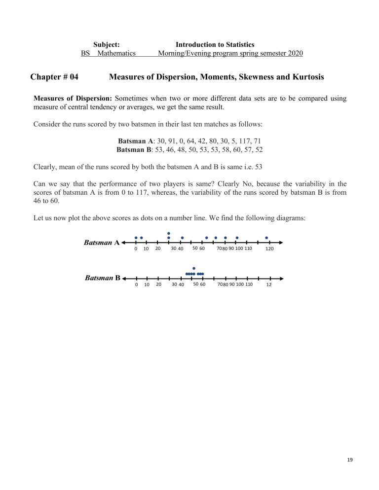
BS
Chapter # 04
Subject:
Mathematics
Introduction to Statistics
Morning/Evening program spring semester 2020
Measures of Dispersion, Moments, Skewness and Kurtosis
Measures of Dispersion: Sometimes when two or more different data sets are to be compared using
measure of central tendency or averages, we get the same result.
Consider the runs scored by two batsmen in their last ten matches as follows:
Batsman A: 30, 91, 0, 64, 42, 80, 30, 5, 117, 71
Batsman B: 53, 46, 48, 50, 53, 53, 58, 60, 57, 52
Clearly, mean of the runs scored by both the batsmen A and B is same i.e. 53
Can we say that the performance of two players is same? Clearly No, because the variability in the
scores of batsman A is from 0 to 117, whereas, the variability of the runs scored by batsman B is from
46 to 60.
Let us now plot the above scores as dots on a number line. We find the following diagrams:
Batsman A
Batsman B
0
10
20
30 40
50 60
7080 90 100 110
120
0
10
20
30 40
50 60
7080 90 100 110
12
19
We can see that the dots corresponding to batsman B are close to each other and is clustering around the
measure of central tendency (mean), while those corresponding to batsman A are scattered or more
spread out. Thus, the measures of central tendency are not sufficient to give complete information about
a given data. In such a situation the comparison becomes very difficult. We therefore, need some
additional information for comparison, concerning with, how the data is dispersed about (more spread
out) the average. This can be done by measuring the dispersion. Like „measures of central tendency‟ we
want to have a single number to describe variability. This single number is called a ‘measure of
dispersion’.
Dispersion: “The v a r i a b i l i t y ( s p r e a d ) t h a t e x i s t s b e t w e e n t h e v a l u e o f a d a t a i s c a l l e d
di spersion ”
OR
“The extent to which the observations are spread around an average is called dispersion or
scatter ”.
As we know that, there are quite a few ways of measuring the central tendency of a data set i.e. A.M,
G.M, H.M, Mode and Median. Similarly, we have different ways of measuring and comparing the
dispersion of the distribution(s). There are two important types of measures of dispersion.
 Types of Measures of Dispersion:
 There are two types of measure of dispersion
I) Absolute Measure of Dispersion
II) Relative Measure of Dispersion
 Absolute Measure
of
Dispersion:
“An absolute measure of dispersion measures the
e.g. if the units of the data are Rs, meters, kg,
etc. The units of the measures of dispersion will also be Rs, meters, kg, etc.
variability in terms of the same units of the data”
The common absolute measures of dispersion are:
 Range
 Quartile Deviation or Semi Inter-Quartile Range
 Average Deviation or Mean Deviation
 Standard Deviation

Relative Measure of Dispersion: “A relative measure of dispersion compares the variability
of two or more data that are independent of the units of measurement”
 In
other
word “A relative measure of dispersion, expresses the absolute measure of dispersion
relative to the relevant average and multiplied by 100 many times” i.e.
20
Relative Dispersion 
Relative Dispersion 
Absolute Dispersion
Average
Absolute Dispersion
Average
100
This is a pure number and independent of the units in which the data has been expressed. It is used for
the purpose to compare the dispersion of a data with the dispersion of another data.
The common relative measures of dispersion are:




Coefficient of Dispersion or Coefficient of Range
Coefficient of Quartile Deviation
Coefficient of Mean Deviation
Coefficient of Standard Deviation or Coefficient of Variation (C.V)
The major difference b/w Absolute and Relative Measures of Dispersion is that the Absolute measure of
dispersion measures only the variability of the data, further it has the unit of measurement; on the other
hand Relative measure of dispersion is used to compare the variation of two or more distributions,
further it is unit less.

Range: “The difference between the l a r g e s t a n d t h e s m a l l e s t v a l u e in a s e t o f d a t a i s
called range ”
OR
“In continuous grouped data the difference between the upper class boundary of the highest
class and lower class boundary of the lowest class is called range”
Formula:
R = Xm – X0 OR R=Largest value –smallest value
Where R is the range, Xm is the largest value and X0 is the smallest value.
 Coefficient of Range or Coefficient of Dispersion: The coefficient of range or coefficient of
dispersion is a relative measure of dispersion and is given by:
Coefficient of Range=
 Numerical example of Range and Coefficient of range
Xm - X0
Xm+ X0
Ex # The marks obtained by 9 students are given below:
xi
45
32
37
46
39
36
41
48
36
21
R  Xm  X0
X m =48,
X 0 =32
R  48  32  R  16 marks
 Coefficient of Range
C.o. f 
C.o. f 
 Quartile
Deviation
or
Xm  X0
Xm  X0
48  32
16
 C.o. f 
 C.o. f  0.2
48  32
80
Semi-inter-quartile
Range:
“half of the difference between the
upper quartile and lower quartile is called the semi-inter quartile range or quartile
deviation”i.e.
Quartile deivation 
Q3  Q1
2
 Coefficient of Quartile Deviation: The coefficient of quartile deviation is a relative measure of
dispersion and is given by:
Coefficient Q.D 
Q3  Q1
Q3  Q1
 Numerical example of quartile deviation and coefficient of quartile deviation
Ex # calculate quartile deviation and coefficient of quartile deviation for ungrouped data.
The marks obtained by 9 students are given below
45
xi
32
37
46
39
Quartile deviation 
“n=9” is odd then we use odd case formulae
36
41
48
36
Q3  Q1
2
th
 n  
Q1  Marks obtained by    1 student
 4  
Quartile deviation 
 Coefficient of Quartile deviation:
Q1 =36 marks, Q3 =45
45  36
 4.5 marks
2
(Answer).
22
Cofficient of Q.D 
Cofficient of Q.D 
Q3  Q1
Q3  Q1
45  32
 0.11
45  32
(Answer).
Ex # calculate quartile deviation and coefficient of quartile deviation for continuous grouped data.
Class boundaries
Midpoints  xi 
29.5---39.5
34.5
8
8
39.5---49.5
44.5
87
95
49.5---59.5
54.5
190
285
59.5---69.5
64.5
304
589
69.5---79.5
74.5
211
800
79.5---89.5
84.5
85
885
89.5---99.5
94.5
20
905
Frequency
n
f
i 1
i
 fi 
Cumulative frequency
 c. f 
=905
h n

  C   Q1  56.40 marks
f 4

h  3n

Q3  l    C   Q3  73.76 marks
f  4

Q1  l 
Calculate Quartile deviation and coefficient of quartile deviation from above results?

Mean Absolute Deviation or Mean Deviation (Average Deviation): “ T h e a r i t h m e t i c m e a n o f
the absolute deviation from an average (mean, median etc.) is called mean
deviation or average deviation”
Coefficient of Mean Deviation: The coefficient of mean deviation is a relative measure of dispersion
and is given by:
23
 Numerical example of Mean deviation and Coefficient of Mean deviation for both ungrouped and
grouped data.
 Calculate the mean deviation and coefficient of mean deviation from (i) the mean, (ii) the median , in
the ungrouped data case, of the following set of examination marks:
45
xi
32
37
46
48
39
36
36
41
n= 9
xi
32
36
36
37
39
41
45
46
48
 xi =360
x
x
i
n
=
xi  x ,
x  40
8
4
4
3
1
1
5
6
8
xi  median ,
xi  x

8
4
4
3
1
1
5
6
8
xi  x
= 40

median  39
7
3
3
2
0
2
6
7
9
xi  median =39
360
=40 marks ,
9
th
 n 1
Median  marks obtained by 
 student
 2 
 Mean deviation from mean is given by
M .D 
 x x
i
n
 M .D 
Median  39 marks
40
 M .D =4.4 marks
9
(Answer).
 Mean deviation from median is given by
 xi  median  M .D  39  M .D =4.3 marks
M .D 
n
9
(Answer).
24
 Calculate coefficient of mean deviation for both mean and median.
4.4
M .D
 C.o.M .D 
 C.o.M .D =0.11 (Answer).
40
mean ( x )
M .D
4.3
C.o.M .D 
 C.o.M .D 
 C.o.M .D =0.11
(Answer).
median
39
C.o.M .D 
 Calculate mean deviation and coefficient of mean deviation from mean in continuous grouped case,
showing the weights of 60 apples.
Weights
(grams)
Frequency
65--84
85--104
105--124
125--144
145--164
09
10
17
10
05
Weight
(grams)
Midpoints
( xi )
Frequency
( fi )
f i xi
65----84
74.5
09
85----104
94.5
105----124
165--184 185--204
04
05
xi  x
f i xi  x
670.5
 48.0
432.0
10
945.0
 28.0
280.0
114.5
17
1946.5
 8.0
136.0
125----144
134.5
10
1345.0
145----164
154.5
05
772.5
165----184
174.5
04
698.0
185----204
194.5
05
972.5
120.0
12.0
160.0
208.0
32.0
360.0
52.0
72.0
n

i 1
x
fx
f
i i
x
i
M .D 
 f x x
f
i
i
i
f i  60
n
fx
i 1
i i
f

i
xi  x
= 1696.0
7350.0
7450.0
 x =122.5 grams
60
 M .D 
1696.0
 M .D =28.27 grams
60
(Answer).
25
Standard Deviation: “The positive square root of v a r i a n c e i s c a l l e d a s s tandard d e v i a t i o n ” .
OR
“The
mean
positive
square
root
of
the
arithmetic
mean
of
the
squared
deviations
from
the
is called the s t a ndard deviation”
 Methods of Calculating Variance and Standard Deviation.
Coefficient of Standard Deviation OR Coefficient of Variation: The coefficient of standard deviation is
a relative measure of dispersion and is given by:
Coefficient of S.D  Standard Deviation
Mean
The coefficient of standard deviation is also called the coefficient of variation, denoted by C.V and is
given by:
26
Standard Deviation  100
C.V 
Mean
27
Coefficient of Variation was introduced by Karl Pearson. It is used to compare the
variation or to compare the performance of two sets of data. A large value of C.V
indicates that there is greater variability and vice versa. Similarly, the smaller the
C.V the more consistent is the performance and vice versa.
 Numerical example of Standard deviation (S.D),Variance and Coefficient of
Variation (C.V) in case of ungrouped data, using direct method:
Ex # Calculate the variance, S.D and C.V from the following marks obtained by 9
students.
45
xi
xi
xi  x
45
5
37
46
48
39
36
 xi  x 
36
25
2025
64
1024
37
3
09
1369
36
2116
6
39
1
01
1521
36
4
16
1296
41
1
01
1681
48
8
64
2304
16
1296
4
 x =360
i
x  x 
i
2
=232
360
 x =40 marks
n
9
2
 xi  x 
232

2
 S 2 =25.78
 S2 
Variance or S 
9
n
i
xi2
2
8
36
x
41
32
46
x
32
x
2
i
=14632
x
Standard deviation or S.D or S 
(Answer).
Using the alternative method.
Calculate Variance:
x  x 
i
n
 marks 
2
2
 S  25.78  S =5.08 marks
28
S
2
x

2
i
n
  xi
 
 n
 S 2 =25.78



2
14632  360 
S 


9
 9 
2
2
 marks 
 S 2 =1625.78  1600
2
(Answer).
Calculate Standard deviation:
S
x
2
i
n
  xi
 
 n



2
2
14632  360 
S

  S  25.78
9
 9 
 S =5.08 marks
(Answer).
 Calculate Coefficient of Variation (C.V):
S .D
5.08
C.V 
100  C.V 
 100  C.V =12.70
x
40
(Answer).
 Calculate the Variance, Standard deviation and Coefficient of Variation
from the following weight of 60 apples in Continuous grouped data:
Weight
(grams)
Midpoints ( xi )
Frequency
( fi )
f i xi
65----84
(65  84) 2  74.5
09
9  74.5=670.
f i xi2
49 952.25
85----104
94.5
10
5
89 302.50
105----124
114.5
17
945.0
222 874.25
125----144
134.5
10
1946.5
180 902.50
145----164
154.5
05
1345.0
119 351.25
165----184
174.5
04
772.5
121 801.00
185----204
194.5
05
698.0
189 151.25
972.5
n

i 1
f i  60
n

i 1
f i xi  735
fx
2
i i
 973 335.00
0.0
Calculate Variance:
2
  f i xi 
S

  f 
i
i 

2
 S  16222.25  15006.25
2
fx

f
2
i i
 S 2 =1216
 grams 
2
973335.00  7350.0 
S 


60
 60 
2
2
(Answer).
Calculate Standard deviation:
29
S
fx
f
2
i i
i
  f i xi

 f
i




2
 S  1216  S =34.87 grams
Calculate Coefficient of Variation:
S .D
34.87
C.V 
100  C.V 
 100  C.V =28.46
x
122.5
(Answer).
(Answer).
Question # Calculate Variance, Standard deviation and Coefficient of Variation using
direct, shortcut and step deviation method for Continuous grouped data, the data are
given below:
Income
Frequency
35--39
13
40--44
15
45--49
17
50--54
28
55--59
12
60--64
10
65--69
05
30
31

Moments: “The arithmetic mean of the rth power of deviations taken
either from mean, zero or from a n y a r b i t r a r y origin (provisional , m e a n)
a r e c a lled moments”.

When the deviations are computed from the arithmetic mean, then such
moments are called moments about mean (mean moments)
or
sometimes called central moments, denoted by mr and given as
follows:
32
 Numerical example of first Moments:
 Calculate first four moments about mean for ungrouped data for the following set
of examination marks:
General formula for moment about mean are given below:
mr
x  x 

r
i
, where r=1, 2, 3, 4.
n
Put r=1
m1
x  x  ,

i
m3
x  x 

m4
x  x 

3
i
n
put r=2
m2
x  x 

i
n
2
,
put r=3
and put r=4
n
4
i
n
33
xi
xi  x
 xi  x 
32
8
64
 512
4096
36
4
16
 64
256
36
4
16
 64
256
37
3
09
 27
81
39
1
01
1
1
 xi  x 
2
 xi  x 
3
41
1
01
1
1
45
5
25
125
625
46
6
36
216
1296
48
8
64
512
4096
 x =360   x  x 
i
x  x 
i
=0
m1 = 0 , m2 = 25.78 (marks)2,
(Answer).
x  x 
2
i
x  x 
3
i
=232
4
4
i
= 186
= 10708
m3 = 20.67 (marks)3 , m4 = 1189.78 (marks)4
 Question # Calculate first four moments about mean for grouped data (using a
continuous grouped case formula). The following distribution relates to the
number of assistants in 50 retail establishments, the data are given below:
No. of
assistants
0
1
2
3
4
5
6
7
8
9
f
3
4
6
7
10
6
5
5
3
1
Using these formulae
m1
 f x  x 

f
 f x  x 

f
i
i
,
m4
i
i
i
i
i
m2
 f x  x 

f
2
,
m3
 f x  x 

f
i
i
3
and
i
4
i
i
 Numerical example of Moment in continuous grouped data:
 Compute the first four moments and measure of Skewness and Kurtosis for the
following distribution of wages using a short cut method:
34
Weekly earnings 5
(Rupees)
6
7
8
9
No. of men
2
5
10
20
1
10
51
11
22
12
13
11
5
14
15
3
1
f i Di
f i Di2
f i Di3
f i Di4
fi
Di   xi  A 
A  10
5
1
5
5
25
 125
625
6
2
4
8
32
 128
512
7
5
3
 15
45
 135
405
8
10
2
 20
40
 80
160
9
20
1
 20
20
 20
20
10
51
0
0
0
0
0
11
22
1
22
22
22
22
12
11
2
22
44
88
176
13
5
3
15
45
135
405
14
3
4
12
48
192
768
15
1
5
5
25
125
625
Earnings
in Rs.
( xi )
Men
f
i
1
i
i
i
8
 m1 
 m1 =0.06,
131
2.64
m3 
fD
f
3
i
i
i
2
i
i
=34
6
fD
m 
f
i
 fD =8  fD
=131
 m3 
i
74
 m3 = 0.56,
131
2
m4 
fD
f
4
i
i
3
i
=7
fD
i
346
 m2 =
131
 m4 
3718
131
 m2  2.64   0.06 
2
2
 m2 = 2.64;
m3  m3  3m2 m1  2 m1 
 m3  0.56  3  2.64  0.06   2 0.06 
3
m4  m4  4m3m1  6m2 m1   3 m 
2
3
 m3 = 0.08;
4
 m4  28.38  4  0.56 0.06   6 2.64 0.06   3 0.06 
2
 m4  28.30
4
i
=3718
 m2 
i
m2  m2   m1 
(always zero),
2
i
i
 m4 =28.38
m1  m1  m1  0
i
4
fD
m 
f
i
fD
4
(Answer).
35
 Calculate measure of Skewness:
b1 
m3
0.08
 b1 
2
3
m2
 2.64 
 b1 =0.0114
(Answer).
 Calculate measure of Kurtosis:
b2 
m4
m22
 b2 
28.30
 2.64 
2
 b2 = 4.0604
(Answer).
Question # Calculate first four moment about the mean and Measure of Skewness
and Kurtosis for the following data are given below,
Using a step deviation method for grouped data?
Age nearest
birth day
22
27
32
37
42
47
52
No. of men
1
2
26
22
20
15
14
36
37
38
39
40
41
42
43