Genealogy in the Era of Genomics

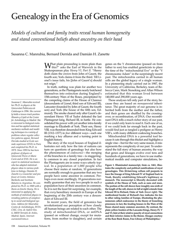
Genealogy in the Era of Genomics
Models of cultural and family traits reveal human homogeneity
and stand conventional beliefs about ancestry on their head
Susanna C. Manrubia, Bernard Derrida and Damián H. Zanette
W
Susanna C. Manrubia received
her Ph.D. in physics at the
Universitat Politècnica de
Catalunya in 1996. She currently holds a tenure-track position
(Ramón y Cajal) at the Center
for Astrobiology in Madrid. She
is interested in biological evolution and has applied statisticalmechanics methods and modeling techniques to a variety of
problems where regular collective patterns appear. Bernard
Derrida studied at École normale supérieure (ENS) in Paris
and completed his Ph.D. in
1979. Since 1993 he has been
professor of physics at
Université Pierre et Marie
Curie and at ENS. He is an
expert in statistical mechanics
who has adapted statisticalphysics ideas to various problems in biology. Damián H.
Zanette is a researcher and professor at Centro Atómico
Bariloche and Instituto
Balseiro in Argentina. He completed his Ph.D. in 1989 with a
thesis on kinetic theory. He is
interested in applying the
methods of statistical physics to
revealing patterns of complexity in social and biological systems. Address for Manrubia:
Centro de Astrobiología, INTACSIC, Ctra. de Ajalvir Km.
4, 28850 Torrejón de Ardoz,
Madrid, Spain. Internet:
[email protected]
158
hat plain proceeding is more plain than
this?” asks the Earl of Warwick in the
Shakespearean play Henry VI, Part II. “Henry
doth claim the crown from John of Gaunt, the
fourth son; York claims it from the third. Till Lionel’s issue fails, his [John of Gaunt’s] should
not reign.”
In truth, nothing was plain for another two
generations, as the Plantagenets nearly butchered
themselves into extinction during England’s
15th-century Wars of the Roses, precipitated by
the competing claims of the House of Clarence
(descendants of Lionel, third son of Edward III),
Lancaster (founded by John of Gaunt, the fourth
son) and York (the house of the fifth son, Edmund). The smoke cleared only after Gaunt’s descendant Henry VII of Tudor defeated the last
Plantagenet king, Richard III, in battle. He consolidated his power with yet another intra-family
marriage to Elizabeth of York. Their son, Henry
VIII, was therefore descended from King Edward
III (1312–1377) in four different ways—each one
marking a key alliance and a turning point in
English history.
The story of the royal houses of England illustrates not only how the fate of nations can
turn on questions of genealogy but also how
the phenomenon of coalescence—the merging
of the branches in a family tree—is staggeringly common in any closed population. In fact
the Plantagenets are in some ways utterly typical. In a population of 1,000 people who
choose their mates at random, 10 generations
are normally enough to guarantee that any two
people have some ancestor in common. Perhaps even more startlingly, 18 generations normally guarantee that any two people in such a
population have all their ancestors in common.
So it is not the least bit surprising, for example,
that every hereditary monarch in Europe at the
beginning of the 20th century was a descendant of Edward III.
In recent years, the field of genomics has
revolutionized our perception of how closely
all human beings are related to each other. The
study of mitochondrial DNA, or mtDNA
(passed on without change, except for mutations, from mother to daughter), and certain
American Scientist, Volume 91
genes on the Y chromosome (passed on from
father to son) has enabled geneticists to place
the time of the “mitochondrial Eve” or the “Y
chromosome Adam” in the surprisingly recent
past. The mitochondria carried in all human
cells are the global legacy of a single woman.
In a pioneering study carried out in 1987, the
University of California, Berkeley, team of Rebecca Cann, Mark Stoneking and Allan Wilson
estimated that this woman lived between
140,000 and 290,000 years ago.
These analyses tell only part of the story, because they are based on monoparental inheritance. The great majority of our genome is inherited both from the mother and the father,
and their genes are shuffled by the crossingover, or recombination, of DNA. Our recombinant DNA tells a much richer story of our past,
if we could only learn to read it. Each one of us,
if we could look far enough back in the past,
would find just as tangled a pedigree as Henry
VIII’s, with many different coalescing branches.
Mitochondrial DNA is a powerful tool because it cuts through this thicket and highlights a
single vine—but for the very same reason, it misrepresents the complexity of our past. To understand the full story of human ancestry, the way
that genes and lineages evolve over tens and
hundreds of generations, we have to use mathematical models and computer simulations, beFigure 1. Illuminated manuscript, from ca. 1461, illustrates the complexity and political ramifications of royal
genealogies. This 20-foot-long vellum roll purports to
trace the lineage of King Edward IV of England back to
Noah, thereby establishing Edward’s legitimacy as
monarch. The manuscript is liberally decorated with
symbols of the House of York, such as suns and roses.
The portion of the roll shown here (roughly one-sixth of
the length of the roll, shown in full at right) extends from
Edward III to Richard, Duke of York (lower right). The
multicolored border of Richard’s box indicates his ties
to other ruling families of Europe, illustrating the phenomenon called coalescence in the theory of branching
processes; in fact, the feuding houses in the Wars of the
Roses shared many common ancestors. By contrast, the
plain yellow borders of the Lancaster Kings, Henry IV, V
and VI, hint at their relative paucity of royal connections
and their inferior claims to the throne. (Images courtesy
of the Rare Book Room, Free Library of Philadelphia.)
2003
March–April
159
Edward III
(1312–1377)
House of Lancaster
John of Gaunt
(1340–1399)
House of York
House of Clarence
Edmund
(1341–1402)
Lionel
(1338–1368)
illegitimate
Henry IV
(1367–1413)
John Beaufort
(1373–1410)
Joan Beaufort
(1379–1440)
unification
of houses
of Clarence
and York
Richard
(1376–1415)
Henry V
(1387–1422)
Roger Mortimer
(1374–1389)
Anne Mortimer
(1390–1411)
John Beaufort
(1404–1444
Cecily
C
il Neville
N ill
(1415–1495)
Henry VI
(1421–1471)
Phillippa
(1355–1389)
Margaret Beaufort
(1441–1509)
Henry VII
(1455 1509)
(1455–1509)
unification of houses
o Lancaster and Yorkk
of
(1411–1460)
Edward IV
(1442–1483)
Wars of
the Roses
House of Tudor
(1466–1503)
(1466
1503)
Henry VIII
(1491–1547)
Figure 2. Highly simplified genealogy of England’s King Henry VIII shows four ancestral lines that lead back to King Edward III. Genealogical coalescence occurs when both of an individual’s parents share a common ancestor. In the pedigree shown here, there were three such marriages. These
were highly nonrandom events, calculated for political effect; the Wars of the Roses were both precipitated and resolved by such unions. However,
the authors’ research shows that coalescence occurs surprisingly rapidly in all closed populations, even those where breeding takes place at random.
cause we do not have genealogical records that
extend so far back into the past. These biparental
models show that mitochondrial DNA actually
underestimates how quickly human populations
become homogeneous in ancestry.
The Extinction of Families
The first serious attempt to solve a genealogical problem mathematically resulted from a
controversy involving one of the most famous
British scientists of the Victorian era, Sir Francis
Galton. Appropriately enough, Galton, a first
cousin of Charles Darwin, had written a book
entitled Hereditary Genius, in which he attempted to explain the oft-noted phenomenon
of the decline of great families. “The instances
are very numerous in which surnames that
were once common have since become scarce
or have wholly disappeared,” Galton wrote
several years later. “The tendency is universal,
and, in explanation of it, the conclusion has
been hastily drawn that a rise in physical comfort and intellectual capacity is necessarily accompanied by diminution in ‘fertility.’” Galton
himself proposed an alternative explanation
that (not surprisingly, for that era) blamed the
women. Men who had recently been elevated
in status, he wrote, would tend to consolidate
160
American Scientist, Volume 91
their positions by marrying heiresses, who
were by definition women from families with
no sons. Such women, he believed, would
themselves be less likely to produce sons.
However, a Swiss botanist named Alphonse
de Candolle correctly pointed out that there was
another possible explanation for the failure of
some family names to perpetuate themselves: It
could simply arise by chance. Until scientists
knew the likelihood of a surname dying out by
random processes, they would not have any
way to tell whether the extinction of “famous”
surnames was in any way anomalous.
In 1874, Galton enlisted a mathematician,
the Reverend Henry William Watson, to resolve this question. The approach Watson took
was ingenious, and he came within a whisker
of discovering a basic result of the 20th-century
theory of branching processes.
Because he wanted to assess the role of
chance, Watson assumed that all males had the
same innate fertility, so that the differences in
their numbers of offspring were attributable
purely to chance. Thus, each male had a certain
probability p0 of having no sons; a probability p1
of having one son; a probability p2 of having
two sons; and so forth. Of course, if a man had
no sons, his lineage would die out immediately.
So the probability of extinction after one generation—call it q1—would be just the same as p0.
But things get more complicated in the succeeding generations, and that is why Galton had
asked for help. For example, a man could have
one son (probability p1) who himself had no sons
(with probability p0); the probability of his line
going extinct in this way would then be the product of the probabilities, p1p0. Or he could have
two sons (with probability p2), who both had no
sons (with probability p02); the probability of this
event would be p2 p02. Adding up the probability
of each of these events gives the probability that
the lineage is extinct after two generations, q2:
q2 = p0 + p1 p0 + p2 p02 + p3 p03 …
Watson’s brilliant insight was that the expression on the right side of this equation,
called the generating function, contained all the
information about the probability of extinction
in later generations as well. Computing the
probabilities of extinction was simply a matter
of applying the generating function over and
over again. Mathematically, he defined the
generating function f(x) by replacing each p0
(except the first) with a variable x:
f(x) = p0 + p1 x + p2 x2 + p3 x3 …
Then he showed the extinction probabilities for
each generation are obtained by feeding the previous generation’s extinction probability back
into this function, a process called iteration:
q1 = f(0), q2 = f(q1), q3 = f(q2), …
And what would be the probability of extinction
after an indefinite number of generations, q∞? It
would simply be an iterate of itself! That is,
f(q∞) = q∞
This is the equation that gives the probability that
any lineage will ultimately—whether after one
generation, 10, or any number—become extinct.
Now, having come so close to a beautiful solution, Watson made his great blunder. With
no demographic data to tell him the probabilities of having zero sons, one son, etc., he simply took a guess: f(x) = (3 + x)5/45. The guess
was not a bad one, but then he made a mathematical mistake by overlooking a solution to
his equation. He thought that the only solution
was f(1) = 1; in other words, q∞ = 1, meaning a
100 percent probability that any lineage will
eventually go extinct. How depressing! “All
the surnames, therefore, tend to extinction in
an indefinite time,” Watson wrote. “This result
might have been anticipated generally, for a
surname once lost can never be recovered, and
there is an additional chance of loss in every
successive generation.”
Watson’s analysis was correct for shrinking
or constant-size populations. But in a growing
population, a second solution for q∞ appears.
For the generating function Watson used,
where the population was growing at a rate of
around 8 percent per generation, it turns out
that f(0.55) = 0.55 as well, meaning there is a 55
percent probability that any lineage will become extinct and a 45 percent probability that
it will survive forever. Very roughly, one may
say that a lineage (say, the Smiths or the Joneses) can reach a critical mass where its survival
is essentially assured. But because Watson
seemed to have resolved the debate, no one
caught his mistake for another 50 years.
Surnames and Mitochondria
In the 1920s, a new generation of biologists and
mathematicians laid the foundations of population genetics, and soon discovered Watson’s error. In a growing population, any given lineage
has a nonzero chance to survive indefinitely. In
1939, Alfred Lotka used data from the 1920 U.S.
census to estimate p0, p1, etc., and then computed that q∞ = 0.819. This meant that in the United
States of that era, the probability for indefinite
survival of a surname, beginning with one
progenitor, was about 18 percent. Or, if you prefer to look at it pessimistically, the probability of
eventual extinction was about 82 percent.
There is always an inherent danger in such
pronouncements: They begin to sound like absolute truths. It is important to remember that
they are dependent on particular mathematical
assumptions, which may or may not conform
to the real world. In Watson’s model, which
has become known to population geneticists
as a Galton-Watson process, some of the
assumptions are quite debatable. Do all males
really have the same innate fertility? Perhaps
being a member of a particular family confers
some evolutionary advantage; in that case, the
process is no longer “neutral.” (This becomes
more likely when one applies Galton-Watson
processes to biological traits rather than surnames.) Is the fertility of each male really independent of each other male, and unvarying
over time? And what happens if we allow
“mutation” of surnames, either through immigration or through fluidity in spelling?
Different cultures, in fact, show great differences in the mutability of surnames. In China,
surnames have been strongly conserved over
thousands of years. A survey by Emperor Tang
Taizong in 627 A.D. found a total of 593 different
surnames. In 960 A.D., the book Surnames of a
Hundred Families recorded 438 surnames. Today,
about 40 percent of the population of China
have one of the 10 most common names, and 70
percent have one of the 45 most common
names. We believe that this lack of mutability is
inherent to the Chinese writing system, which
represents each surname by a single character.
By contrast, America and Canada have the
highest diversity of surnames in the world, a
legacy of their history as countries built by immigration. The extreme mutability of English
Medieval heraldic
emblems of royal
lineage from the
Edward IV roll:
Rose(facing page),
(top to bottom above)
crown, the black bull
of Clare (House of
Clarence) and Edward
IV’s mèlange of royal
symbols: falcon, fetterlock, rose and cross of
St. George.
2003
March–April
161
spellings has also increased the variety of surnames, as the following excerpt from a World
Wide Web page devoted to Hemingways (Figure
3 below) attests:
My most elusive Hemingway ancestor,
Fisher Hemingway, born in 1819 or 1820 in
New York… is listed as: Hemensway, Fisher in the 1880 census; Hemingway, Fisher
when he married Catharine Chambers in
1858; Hemenway, Fisher in the 1845-46
Cleveland city directory; Henenway, Fisher
in the 1840 census; Hemmingway, Fisher
when he married Elizabeth Elliott in 1839
… My current list of Hemingway variations runs to many pages, and I suspect
that I have overlooked many others.
We have studied the distribution of surnames using a simple model that allows for a
small probability of mutations at any time and
that also includes a flexible death rate that can
be made equal to, greater than or less than the
birth rate. In this model, like the Galton-Watson model, we find dramatic differences between growing populations and static ones,
where the birth and death rate are equal.
Kemmingway
Hemenwry
Kemingway
Heneway
Hemenwary
Hemmingway
Hemensway
Hemingway
Hiningway
Heminway
Hemenway
Hememway
Huminway
Emingway
Himingway
Henenway
Heningway
Hemmenway
Hemanway
Heninway
Hemaway
Homanway
Hemanyway
Hininway
Hamanway
Figure 3. Spelling of English surnames has historically been very flexible. A small and
by no means complete set of variations of the name “Hemingway” is shown here,
along with the paths of mutation that change one variant to another. (These are actual
variations that appeared in U.S. Census records from the 1800s.) The authors have
studied a model of surname inheritance that includes a small but nonzero probability that any name will mutate when passed to the next generation. This model predicts
that mutations will ensure an ever-increasing diversity of surnames in any growing
population (but a shrinking number of surnames in a stable population). In a society
such as China, where the mutation rate of surnames is essentially zero, surname diversity has changed very little over the centuries.
In a growing population, the diversity of
names always increases over time. Given enough
time, the number of names that belong to exactly
y people, or n(y), becomes proportional to 1/y2
for large enough y, that is to say for large family
sizes. Thus, for example, there should be 100
times as many names that belong to only 20 people as names that belong to 200 people.
162
American Scientist, Volume 91
In a static population, on the other hand, the
mutation rate becomes very important. If the mutation rate is too low, then the diversity is very
likely to decrease until there is only one dominant surname. On the other hand, if the mutation
rate is high, then the frequency function n(y) will
approach a steady state, but one that is much
more biased toward small family sizes than is the
distribution for a growing population.
We emphasize that these steady-state distributions hold true only after many generations.
On the flip side of the coin, deviations from the
expected steady state can reflect recent historical
events. For instance, modern Japanese surnames began to appear only 120 years ago.
Thus we would expect the distribution of family sizes—particularly large families—to retain
an imprint of the “initial state” of a century ago.
A comparison with real data taken from
three sources—the whole 1996 Argentine
phone book, the “A” entries of the 1996 Berlin
phone book, and the whole list of surnames
from five Japanese cities circa 2000—seems to
bear out these conclusions. (In this study we
defined a “family” as all people with the same
last name.) The Argentine data fit very nicely
to the steady-state line n(y), except for a slight
deficit of very large families. This is consistent
with Argentina’s demography, a generally
pan-European population that has been disturbed a bit by immigration in the late 1800s
and after World War II. The Berlin data have
more scatter, because they come from a smaller
data set, but seem to follow the steady-state
distribution. The Japanese data, however, deviate from the steady-state distribution dramatically, with a significant excess of large
families. If we were to return a century or two
from now, we would probably find the distribution to be clustered more closely around the
straight line shown in Figure 4. However, this
prediction would not hold up if Japan (or either of the other countries) went through a prolonged period of zero population growth.
Modern scientists may not care as much as
Victorian scientists did about surnames or the
death of “great families.” They do, however,
care about mitochondrial DNA, which has the
same mode of inheritance as a surname. A
mother’s mtDNA is passed along intact, except
for rare mutations, to all of her children; only
her daughters, though, can propagate that DNA
to the next generation. The simplest counting
unit on a double strand of DNA is the base pair,
made up of a nucleotide on each strand. There is
a special segment in mtDNA, the so-called control region, about 500 base pairs in length, that
apparently evolves neutrally. This segment does
not seem to have a specific function, and the
mutations do not offer any survival benefit.
Thus the slow, random genetic drift of mtDNA
forms an excellent genetic clock that indicates
whether two people, or two groups of people,
One Parent or Two?
Mitochondrial DNA has provided groundbreaking insights into the history of humans.
However, mtDNA tells only part of the story:
We know that we have, potentially, as many
contributors to our genes as ancestors in our
genealogical tree. “Mitochondrial Eve” and “Ychromosome Adam” need not be contemporaries or live in the same region, and they are
not necessarily the most important contributors to our genetic makeup. In fact, if we had
one common ancestor at some particular time,
we almost certainly had many of them. Mitochondrial Eve merely happens to be the one
who is our mother’s mother’s mother’s (repeat
this many thousand times) mother. Mitochondrial analysis cannot tell us who is our mother ’s father ’s mother ’s father ’s (repeat this
many thousand times) father. Some of these
undetectable ancestors may have lived a good
deal more recently than mitochondrial Eve.
It is also worth noting that common ancestors do not necessarily make equal contributions
to our genome. It is true that our parents each
contribute 50 percent of our genetic material,
but our grandparents do not necessarily each
contribute 25 percent. Going farther back, some
ancestors may have their genetic contribution
enhanced by genealogical coalescence: More
branches leading to them translates to more opportunities to pass their DNA down to us.
Two recent studies, one by us and the other
by Joseph Chang of Yale University, have emphasized the difference between the genetic
and genealogical approaches to coalescence.
The mathematical models of genealogy that
we studied and that Chang studied are very
similar and can be extended, as we did, to populations of varying sizes. The models work
from present to past. We assume that each in-
10
–1
Argentina
Berlin (×10–1)
surname frequency (log scale)
had a common ancestor, and how long ago. The
discovery of this clock has cleared up some important historical debates, both from the recent
and the distant past. For example, the mtDNA
of a woman whom many people believed to be
the princess Anastasia, the daughter of the last
tsar of Russia, turned out to be unrelated to other living relatives of the Romanov dynasty. The
mitochondria of Pacific Islanders have mutations common among Asiatic people, and thus
prove that the Pacific Islanders came from Asia,
rather than from the Americas as some historians believed. And the analysis of mtDNA from
the upper arm of a 50,000-year-old Neandertal
skeleton established that Neandertals apparently split from the lineage leading to modern human beings some 500,000 years ago and therefore do not contribute mtDNA to modern
humans. In general, mtDNA, just like surnames,
can identify demographic events in a population’s past, such as migrations, population bottlenecks or expansions.
10
–2
10
–3
Japan (×10–3)
10–4
10
–5
10
–6
10–7
1
100
10
1,000
family size (log scale)
Figure 4. Surname model makes precise predictions about the number of names that
will have a given “family size”—that is, about the distribution of family sizes. (Here, for
the sake of simplicity, we define a family to consist of all the individuals with a given
surname.) The graph shows the predicted frequency of each family size in the model
(lines), compared with data from phone books in Argentina (squares), Berlin (circles)
and Japan (triangles). The Berlin and Japan data have been scaled downward for presentation. The family-size distributions for Argentina and Berlin match the model predictions reasonably well, but the Japanese data diverge considerably. The authors believe this reflects the relatively recent introduction of surnames in Japan, which means
that the family-size distribution has not yet reached a steady state.
dividual randomly chooses two parents from
the preceding generation.
“Of course [this model] is not meant to be particularly realistic,” writes Chang. “Still, one might
worry that this simple model ignores considerations of sex and allows impossible genealogies. If
this seems bothersome, an alternative interpretation of the same process is that each ‘individual’
is actually a couple, and that the population consists of n monogamous couples. Then the random choices cause no contradictions: the husband and wife each were born to a couple from
the previous generation.” As further arguments
for the validity of this model, we might add that
it gives a good match to census data on family
sizes, and that it can (if desired) be reformulated
to move forward in time. (The “forward” version
is, however, slightly more complicated.)
With this model, one can study a variety of
questions. For example, there is the one Galton
and Watson were interested in: What is the
probability that your line (now defined as all
descendants, not just sons of sons of sons) will
go extinct? If you pick two people at random in
2003
March–April
163
the present, how many generations back will
you have to go to find a common ancestor?
How far back do you have to go until all the ancestors are the same? Figure 5 illustrates these
questions. In this constant population of 12
people, the first common ancestor of “Sam”
and “Betty” is a grandmother, “Alice,” shown
in red bounded by blue. Going back to previous generations, we find the red+blue common
ancestors becoming more and more common,
until after a mere 6 generations there is complete overlap between Sam’s and Betty’s ancestry. Notice that the mitochondrial lineages
(shown in green) have not yet coalesced, so that
a geneticist studying mtDNA may or may not
realize that Sam and Betty are so closely related.
This example is not unusual. The number of
generations to the first common ancestor, in a
constant population of n people, is typically the
logarithm of n to the base 2. (The logarithm of 12
to the base 2 is 3.6, so we would expect a common ancestor around three or four generations
ago.) According to Chang, the number of generations, G, until any two individuals have the
same set of ancestors, is 1.77 times the logarithm
of n to the base 2. One might call this the “coalescence time” of the population. (For a population
of 12, it works out to about 6.3 generations, which
agrees with the example in Figure 5.) We happened to choose a different approach from
Figure 5. Coalescence in a two-parent model comes about much more rapidly than coalescence in a one-parent model. Each row in this diagram represents one generation in a
constant-sized population of 12 individuals. Two people (“Sam” and “Betty” in the
text) are chosen in the current generation (bottom row), and their ancestors are traced
back for six generations. The most recent common ancestor (red+blue square) appears in
generation 2. In earlier generations, the number of shared ancestors continues to increase, until in generation 6 the red and blue ancestries overlap completely. By contrast,
in types of inheritance that involve a single parent, such as mitochondrial DNA, a common ancestor may not be detected after six generations (green lines).
164
American Scientist, Volume 91
Chang’s, comparing instead the number of times
that a given ancestor appears in two distinct genealogical trees. We found that it takes on the order of log n generations for the number of repetitions of each ancestor to become identical in any
tree, with an abrupt transition of about 14 generations (independent of the population size) where
the similarity jumps from 1 to 99 percent. Finally,
both Chang and our group found that there is
not only a universal common ancestor but a universal ancestral population. At the coalescence time a
complete dichotomy emerges, in which every individual is either an ancestor of all people in the
present generation or none of them. (If the population is constant, about 80 percent of the people
in the Gth generation are universal ancestors, and
the remaining 20 percent have had their lines go
extinct. In a growing population, the proportion
of universal ancestors is higher and the proportion of extinct lines is lower.)
Clearly, these model results stand the conventional wisdom about ancestry and “mitochondrial Eves” on its head. It is therefore very
important to scrutinize the assumptions we
made, to see what is reasonable and what is
not. We heartily concur with Chang when he
writes, “What is the significance of these results? An application to the world population
of humans would be an obvious misuse.”
In the real world, the selection of parents (or
in the “forward” model, the selection of mates)
is, of course, not random. Geography, race, religion and class have always played strong
roles in biasing mate selection. Even so, the
models are telling us something important: In
subpopulations where random mating can
take place, a common ancestor pool emerges
with startling rapidity, in hundreds rather than
hundreds of thousands of years.
By contrast, genetic homogeneity in a population takes a great deal longer to emerge. Although a genealogical tree has the property of
doubling the ancestry at each generation, this is
not the case for individual genes, which necessarily are inherited along single branches and
thus conform to a monoparental model. Thus
one might define a genetic coalescence time to be
the number of generations required to reach a
common ancestor for any particular non-recombining allele. (This is essentially the same as the
mitochondrial DNA problem, in which each individual is linked to only one parent.) In his pioneering contribution, Sir John Frank Charles
Kingman, currently at the University of Cambridge, has shown that this kind of coalescence
takes a number of generations equal to the population size itself. Thus, for example, a randomly
intermarrying population of 1,000 people will
reach genealogical coalescence in 18 generations,
but will require a thousand generations to
achieve genetic coalescence. And even in this
case, different genes may lead to different common ancestors. Thus, once again, it is more ap-
one-parent model
two-parent model
1
“similarity”
0.8
population
400
800
1,600
0.6
0.4
population
400
800
1,600
0.2
0
10
20
15
generation in the past
25 0
2,000
4,000
6,000
generation in the past
8,000
10,00
Figure 6. In closed populations with random mating, two-parent models show that complete coalescence of ancestry takes place with startling rapidity. Here two different measures of genealogical “similarity” are used. In a
two-parent model (left), “similarity” represents the probability that an individual has as ancestors the whole population present at generation n in the past. The speed of the transition from universal unrelatedness to universal
relatedness does not depend on population size, although the timing of the transition does (larger populations require more generations.) In a one-parent model, “similarity” represents the probability that all the individuals in
the current population share mitochondrial DNA (for example) from the same person n generations in the past.
For populations of a few hundred people, it takes more than 1,000 generations before there is a large probability that all people have the same mitochondrial ancestor. In this case, the speed of the transition depends on the
population size, and is slower at larger present population sizes.
propriate to speak of an entire ancestral population, rather than a single progenitor Eve.
Conclusion
The analysis of mitochondrial DNA has allowed
scientists to obtain many spectacular results regarding human evolution. MtDNA represents a
small, though essential, piece of our whole
genome. Its relevance to the origin of and relationships among human groups lies in its peculiar mode of transmission through the maternal
line, analogous to surnames. However, our genetic ancestry is much broader, because we know
that a large fraction of any population many generations ago is included in our genealogical tree.
Our surname, like mtDNA, is only one small
piece of information about our origins.
Mitochondrial genes contain information
largely about energy production. But most of
the information that characterizes us as human
beings resides in our so-called nuclear genes,
which constitute more than 99.99 percent of the
human genome. These genes mix every time a
pair of humans reproduce, through the process
of recombination. If we could follow all the
branches through which we have inherited our
genes, we would probably find that all those
people included in our genealogical tree have
contributed—maybe in an extremely diluted
way—to our genetic inheritance. It is not only
mitochondrial Eve, but probably most of her
contemporaries, who have left silent footprints
in our extant (collective) genome.
The next time you hear someone boasting of
being descended from royalty, take heart: There
is a very good probability that you have noble
ancestors too. The rapid mixing of genealogical
branches, within only a few tens of generations,
almost guarantees it. The real doubt is how
much “royal blood” your friend (or you) still
carry in your genes. Genealogy does not mean
genes. And how similar we are genetically remains an issue of current research.
Bibliography
Cann, R., M. Stoneking and A. C. Wilson. 1987. Mitochondrial DNA and human evolution. Nature 325:31–36.
Cavalli-Sforza, Luigi L., P. Menozzi and A. Piazza. 1994.
History and Geography of Human Genes. Princeton, N.J.:
Princeton University Press.
Chang, Joseph T. 1999. Recent common ancestors of all present-day individuals. Advances in Applied Probability
31:1002–1026.
Derrida, Bernard, Susanna C. Manrubia and Damián H.
Zanette. 1999. Statistical properties of genealogical trees.
Physical Review Letters 82:1987–1990.
Derrida, Bernard, Susanna C. Manrubia and Damián H.
Zanette. 2000a. On the genealogy of a population of biparental individuals. Journal of Theoretical Biology
203:303–315.
Derrida, Bernard, Susanna C. Manrubia and Damián H.
Zanette. 2000b. Distribution of repetitions of ancestors in
genealogical trees. Physica A 281:1–16.
Harris, Theodore E. 1963. The Theory of Branching Processes.
New York: Springer Verlag.
Kingman, J. F. C. 1982. The coalescent. Stochastic Processes
and Their Applications 13:235–248).
Manrubia, Susanna C., and Damián H. Zanette. 2002. At
the boundary between biological and cultural evolution: The origin of surname distributions. Journal of Theoretical Biology 216:461–477.
Sykes, Brian. 2001. The Seven Daughters of Eve. New York:
W. W. Norton & Company.
Watson, H. W., and Francis Galton. 1874. On the probability of the extinction of families. The Journal of the Royal
Anthropological Institute 4:138–144.
Zanette, Damián H., and Susanna C. Manrubia. 2001.Vertical transmission of culture and the distribution of family names. Physica A 295:1–8.
Links to Internet
resources for further
exploration of
“Genealogy in the Era
of Genomics” are
available on the
American Scientist
Web site:
http://www.american
scientist.org/
articles/03articles/
manrubia.html
2003
March–April
165