BANDWIDTH REDUCTION ON SPARSE MATRICES BY

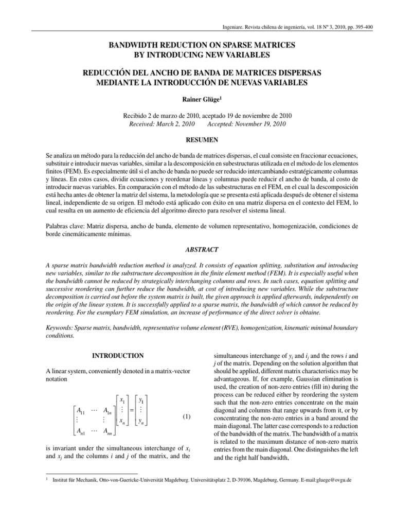
Ingeniare. Revista chilena de ingeniería, vol. 18 Nº 3, 2010, pp. 395-400
BANDWIDTH REDUCTION ON SPARSE MATRICES
BY INTRODUCING NEW VARIABLES
REDUCCIÓN DEL ANCHO DE BANDA DE MATRICES DISPERSAS
MEDIANTE LA INTRODUCCIÓN DE NUEVAS VARIABLES
Rainer Glüge1
Recibido 2 de marzo de 2010, aceptado 19 de noviembre de 2010
Received: March 2, 2010 Accepted: November 19, 2010
RESUMEN
Se analiza un método para la reducción del ancho de banda de matrices dispersas, el cual consiste en fraccionar ecuaciones,
substituir e introducir nuevas variables, similar a la descomposición en subestructuras utilizada en el método de los elementos
finitos (FEM). Es especialmente útil si el ancho de banda no puede ser reducido intercambiando estratégicamente columnas
y líneas. En estos casos, dividir ecuaciones y reordenar líneas y columnas puede reducir el ancho de banda, al costo de
introducir nuevas variables. En comparación con el método de las subestructuras en el FEM, en el cual la descomposición
está hecha antes de obtener la matriz del sistema, la metodología que se presenta está aplicada después de obtener el sistema
lineal, independiente de su origen. El método está aplicado con éxito en una matriz dispersa en el contexto del FEM, lo
cual resulta en un aumento de eficiencia del algoritmo directo para resolver el sistema lineal.
Palabras clave: Matriz dispersa, ancho de banda, elemento de volumen representativo, homogenización, condiciones de
borde cinemáticamente mínimas.
ABSTRACT
A sparse matrix bandwidth reduction method is analyzed. It consists of equation splitting, substitution and introducing
new variables, similar to the substructure decomposition in the finite element method (FEM). It is especially useful when
the bandwidth cannot be reduced by strategically interchanging columns and rows. In such cases, equation splitting and
successive reordering can further reduce the bandwidth, at cost of introducing new variables. While the substructure
decomposition is carried out before the system matrix is built, the given approach is applied afterwards, independently on
the origin of the linear system. It is successfully applied to a sparse matrix, the bandwidth of which cannot be reduced by
reordering. For the exemplary FEM simulation, an increase of performance of the direct solver is obtaine.
Keywords: Sparse matrix, bandwidth, representative volume element (RVE), homogenization, kinematic minimal boundary
conditions.
INTRODUCTION
A linear system, conveniently denoted in a matrix-vector
notation
 A11


A
 n1
 x1   y1 
   
 A1n     =   

   x n   yn 
 Ann 
(1)
is invariant under the simultaneous interchange of xi
and xj and the columns i and j of the matrix, and the
1
simultaneous interchange of yi and ij and the rows i and
j of the matrix. Depending on the solution algorithm that
should be applied, different matrix characteristics may be
advantageous. If, for example, Gaussian elimination is
used, the creation of non-zero entries (fill in) during the
process can be reduced either by reordering the system
such that the non-zero entries concentrate on the main
diagonal and columns that range upwards from it, or by
concentrating the non-zero entries in a band around the
main diagonal. The latter case corresponds to a reduction
of the bandwidth of the matrix. The bandwidth of a matrix
is related to the maximum distance of non-zero matrix
entries from the main diagonal. One distinguishes the left
and the right half bandwidth,
Institut für Mechanik, Otto-von-Guericke-Universität Magdeburg. Universitätsplatz 2, D-39106, Magdeburg, Germany. E-mail:[email protected]
Ingeniare. Revista chilena de ingeniería, vol. 18 Nº 3, 2010
k1 = max(i − j),
i > j,
Aij ≠ 0
(2)
BANDWIDTH REDUCTION BY INTRODUCING
NEW DEGREES OF FREEDOM
k2 = max( j − i),
j > i,
Aij ≠ 0
(3)
Row-Dominant matrices
Consider the linear system
which coincide for symmetric matrices. The bandwidth b
is given by b=k1+k2. Especially direct solution algorithms
can take advantage of a band structure, which is moreover
helpful in reducing the memory requirements. For direct
solvers, tcpu ≈ cb2 holds. Consequently, one is interested in
reordering the linear system such that the system matrix
bandwidth is reduced.
The efficient reordering of linear systems is an important
topic discussed in the literature since sparse linear systems
emerged routinely in engineering applications, i.e. since the
development of the finite difference and the finite element
method and the availability of computers. The reordering
such that b is minimized is a combinatorial problem.
Different algorithms that base on a graph representation
of the non-zero connections of columns and rows have
been proposed. The most common methods are the CuthillMcKee and the Reverse Cuthill-McKee algorithm [6-5],
Sloans ordering [14], Gibbs-Poole-Stockmeyer ordering
[10], minimum degree ordering and nested dissection,
which is also referred to as nested substructure method
in the context of the FEM [7]. A survey is given by [2].
However, there are cases in which the bandwidth cannot
be reduced by reordering. If the linear system consists
mostly of equations with a small number of terms but
at least one equation has a considerably larger number
of terms, the matrix contains dominant non-zero rows,
while the matrix contains dominant non-zero columns
if at least one variable appears much more often in the
equations than the other variables. Such linear systems
are not encountered very often, but they can arise, e.g.,
if a large number of nodes of a finite element mesh is
constrained by few equations. Here, an approach which
permits a further reduction of the bandwidth at the cost
of the overall system size is presented, and tested in
conjunction with the FE system ABAQUS.
 A11





A12
A22
 x1   y1 
   
 A1n     =   
   
  x n   yn 



Ann 
(4)
i.e. a matrix with the first row and the diagonal entirely
filled with non-zero entries, while all other matrix
elements are equal to zero. The bandwidth of the matrix
is equal to n, and one can see that the interchanging of
columns and rows can reduce the bandwidth maximally
to approximately n/2, by putting the dominant row in a
more central position. Let us introduce the substitution
x * = A1m +1 x m +1 + …+ A1n x n
(5)
and treat x* as unknown. Hence, we add the latter equation
to the list of equations and rewrite the system as
 A11











A12  A1m
A22

Amm
Am +1m +1

A1m +1
Ann
 A1n
 x1   y1 
   

 
1   =  

x
yn 
 n
 *  
  x   0 







−1
(6)
The matrix bandwidth can now be reduced by interchanging
row and columns to approximately n/4. The new system
has one more degree of freedom, but its minimal bandwidth
is halved. The procedure can be applied to the remaining
dominant rows to reduce the bandwidth to a certain value,
or one can directly split the first equation into p equations,
reducing the bandwidth to approximately n/(2p).
396
R. Glüge: Bandwidth reduction on sparse matrices by introducing new variables
Column-Dominant matrices
A similar strategy can be employed for column-dominant
linear systems. Consider the linear system
 A11

 A21


 An1
A22
 x1   y1 
   
   =   
   
  x n   yn 



Ann 
(7)
x*
The first column can be split up by introducing 1=x1,
and distributing the coefficients that are connected to x1
equally on x1 and x1*. Adding the equation and the new
variable to the system, one obtains
 A11

 A21


 Am1





1
A22

Amm
Am+1m+1

Ann
 x1   y1 
   

 
 =  
  x n   yn 
 *  
  x1   0 


Am+11 



An1 
−1 
(8)
Again, the bandwidth of the latter system can be reduced
by column and row permutation.
PRESERVATION OF SYMMETRY
The latter substitutions can be carried out such that
the symmetry is preserved, which is demonstrated on
a symbolically filled matrix. The vector reordering is
disregarded for convenience. Being given a matrix of
the form
• •

• •
•

•
•

•
•
•
•
•
•
•
•







• 
•

•
•





1

(9)
•
•
•
•
•
•
•
•
•
•





• 
• 

• 
−1
(10)
and then split the dominant row and append the newly
formed column and row,
• • •
1 


• •

•

•


•
•




•
•


• •



1
−1



• • •
−1
(11)
followed by interchanging the newly added columns or
rows (rows here)
•

•
•







1
•
•
•
•
•
•
•
•
•
•
1 




•


•

•

−1

−1
(12)
For large systems, the increase in variables may have no
practical effect at all, converse to the bandwidth reduction.
For the preceding examples, the equation splitting is
more costly than applying Gaussian elimination, after
reordering the matrices such that the fill in is avoided.
However, in some cases, the splitting of dominant rows
and columns can significantly reduce the solution effort.
In the following section an example for the profitable
application of the equation splitting is given.
we firstly split the dominant column and append the newly
formed column and row,
397
Ingeniare. Revista chilena de ingeniería, vol. 18 Nº 3, 2010
EXAMPLE
The finite element method is used to approximate the
solution of a partial differential (PDE) equation by
discretizing the domain by finite elements, which are
connected at nodes. The solution is approximated by
piecewise steady functions inside the elements, the
parameters of which are determined by exploiting the weak
form of the PDE (see, e.g., [1]). The smallest possible
bandwidth of the symmetric system matrix depends
on the number of elements to which the node with the
most connections is connected. The actual bandwidth
depends on the specific structure of the finite element
mesh. Reordering the nodes corresponds to column and
row interchanging. There are geometries for which even
an optimized mesh structure has a large bandwidth. But
even in such cases the bandwidth is usually considerably
smaller than the system size. However, the FEM permits
a connection of nodes not only by the elements, but by
other constraint equations.
Note that in the context of the FEM, the algorithm
demonstrated here is similar to the decomposition of the
FE model into hyper- and substructures. Referring to the
substitution (3), one would say that the nodes belonging
to the xi that are summarized to x* form a substructure.
The procedure discussed here does not operate on nodes
but on degrees of freedom. The most important difference
is that the method presented here is independent on the
problem, i.e. it can be applied algorithmically to any linear
system, while the substructure decomposition is part of the
specific FE modelling. In the substructure decomposition,
the structure is divided into independent substructures,
while the substitution (3) must not be a reasonable division
into independent parts from the engineering point of view.
We encountered the problem when we prescribed the
average displacement u on an entire face of a structure
in a continuum mechanics problem, which results in a
large constraint equation
u1 + u2 + …+ un = nu
(13)
In our case, the constraints emerge in a homogenization
procedure. Homogenization bridges the gap from one
scale to a larger scale. If one knows the constituents of
a microstructure and their material properties, one can
approximate the behaviour on a larger scale by averaging
over the volume on the lower scale (see, e.g., [4] and the
references within). Here, we present a numerical example.
We want to apply an average deformation gradient
398
F=
1
F ( X dV
V Ω∫
)
(14)
to a cubic representative volume element (RVE). Ω
denotes the domain occupied by the body in the reference
placement. F and H are called the deformation and the
displacement gradient, respectively, x and X are the
position vectors of material points in the reference and the
current placement, and u=x-X denotes the displacement
vector. For an account to continuum mechanics see for
example [12, 3].
))
(
)
F = x ( X ⊗∇ X = X + u ( X ⊗∇ X = I + H
(15)
F is commonly enforced by homogeneous or periodic
boundary conditions. These have the drawback that they
stiffen the RVE artificially, as, e.g., shear bands cannot
arrange freely. Here we focus on applying F without
further constraints, which is referred to as the kinematic
minimal boundary conditions [13], natural boundary
conditions [8] or weakly enforced kinematic boundary
conditions [9]. By Gauss theorem we convert the volume
integral into a surface integral,
F=
(
))
1
I + u ( X ⊗∇ X dV
V Ω∫
I+H=
1
1
VI + ∫ u ( X ⊗ n0 dA
V
VΩ
H=
)
1
u ( X ⊗n0 dA
V Ω∫
)
(16)
(17)
(18)
In the FE implementation, the latter integral converts into
a sum over the weighted displacements of the surface
nodes, the weight of which depends on the fraction of the
surface that is assigned to each node. E.g., for hexahedral
elements, which result in quadrilateral surfaces, a fourth of
the surface of each element to which the node is connected
is added. The FE system ABAQUS has been used for the
following example. The FE model consists of a regular
meshed cube (20 elements per edge), linear eight node
bricks (element type C3D8) are used. The corner node
at (0,0,0) is tied, which is the only direct displacement
boundary condition. The deformation is enforced by
prescribing the H as described above. For this purpose,
3 artificial nodes have been created, the 3 degrees of
R. Glüge: Bandwidth reduction on sparse matrices by introducing new variables
freedom of which represent the components of H . In any
case, 9 large constrained equations have to be taken into
account. It remains open whether the artificial nodes are
constrained by a displacement (average straining) or by
a force (average stress). For the comparison between not
splitting and splitting of the equations and for checking of
the implementation, a homogeneous linear elastic isotropic
material behaviour is assumed (St. Venant-Kirchhoff). For
illustration purposes of the boundary conditions, a central
hard spherical inclusion of diameter 0.4*edge length and
Gsphere = 5Gmatrix = Gsphere = 5Gmatrix = 10.000MPa (shear
and compression modulus, respectively) is included by
the Gauss-point method (multiphase elements, see [11]).
With this RVE, a uniaxial tension and a shear test have
been carried out. For the uniaxial tension, H11 = 0.1 and
H12 = H13 = H23 = H21 = H31 = H32 = 0 have been prescribed,
i.e. seven large constraining equations are included. The
components H22 and H33 are not constrained in order to
permit an average lateral straining. For the shear test, H22
and H13 = H23 = H21 = H31 = H32 = 0 haven been prescribed,
while the average normal straining can freely adjust, i.e.
H11, H22 and H33 are not prescribed.
Table 1 gives an overview on the difference between the
FE simulations if carried out with and without equation
splitting. Both simulation give exactly the same results
and convergence behaviour, since the modifications of
the linear system presented here do not affect the results.
However, one can see in Table 1 that the equation splitting
results in a considerable reduction of linear system solver
effort. In Figure 1, the deformed RVE with the spherical
inclusion is depicted. For a review of the FE simulations,
supplementary files are provided at http://www.ovgu.
de/ifme/l-festigkeit/ Rev_chilena_de_eng_supplement_
gluege_2010.zip, including the ABAQUS input files, the
user material subroutine, the iteration log files and the
output databases.
Figure 1. Cross sections of two deformed RVE with a
central spherical inclusion. For the tension test
(top), the displacement is scaled uniformly by a
factor of 10 in order to amplify the deformation.
The greyscaling (12 bands) corresponds to
the equivalent Mises stress, from 400MPa
(white) to 1.200MPa (black). For the shear test
(bottom), the displacement is scaled by a factor
of 2 in the shear direction (d) and the shear
plane normal (n), and by a factor of 20 in the
direction normal to d and n. The greyscaling
(12 bands) corresponds to the equivalent Mises
stress, from 1.000MPa (white) to 2.400MPa
(black). One can see the non-periodicity of
the deformation.
Table 1. Long constraining equations vs. equation
splitting with a direct solver in ABAQUS.
Max. Terms in eq
Deg. Of freedom
Splitting
No splitting
20
2*21²+1=883
28215
3*21³+9=27.792
Floating point ops per
iteration
4.61 E10
4.34 E11
Min. Memory usage
256 MB
853.71 MB
141
1.621
FE sim wallclock
time
399
Ingeniare. Revista chilena de ingeniería, vol. 18 Nº 3, 2010
CONCLUSIONS
The present work points out problems that may emerge
when row- and column-dominant linear systems are
treated by direct solution methods. An efficient treatment
is exemplified on a continuum mechanics problem, namely
a numerical homogenization by the representative volume
element technique, where kinematic minimal boundary
conditions have been employed. Further research may
focus on how the modifications affect the properties of
the linear system. Moreover, it should not be concealed
that the kinematic minimal boundary conditions are not
as commonly employed as the periodic displacement and
the homogeneous displacement boundary conditions,
and have received therefore less attention. In particular,
the question under which circumstances the kinematic
minimal boundary conditions satisfy the Hill condition
[15] is not answered conclusively.
ACKNOWLEDGEMENT
[6]
[7]
[8]
[9]
[10]
I like to express my gratitude to my wife, who reviewed
the Spanish part of this work.
REFERENCES
[1]
[2]
[3]
[4]
[5]
400
T. Belytschko, W.K. Liu and B. Moran. “Nonlinear
Finite Elements for Continua and Structures”. John
Wiley & Sons. New York, USA. 2000.
M. Benzi. “Preconditioning Techniques for
Large Linear Systems: A Survey”. Journal of
Computational Physics. Vol. 182, Issue 2, pp. 418477. November, 2002.
A. Bertram. “Elasticity and Plasticity of Large
Deformations”. Springer Verlag. Berlin, Germany.
2005.
P. Castaneda, J. Telega and B. Gambin. “Nonlinear
Homogenization and its Application to Composites,
Polycrystals and Smart Materials”. Proceedings
of the NATO Advanced Research Workshop,
NATO Science Series II: Mathematics, Physics
and Chemistry 170. Springer. Netherland. 2004.
W. Chan and A. George. “A linear time
implementation of the Reverse Cuthill-McKee
algorith”. BIT Numerical Mathematics. Vol. 20,
pp. 8-14. 1980.
[11] [12]
[13]
[14]
[15] E. Cuthill and J. McKee. “Reducing the bandwidth
of sparse symmetric matrices”. Proceedings of
the 1969 24th National Conference of the ACM,
ACM Press, pp. 157-172. New York, N.Y., USA.
1969.
S.Y. Fialko. “The nested substructure method for
solving large finite-element systems as applied to
thin-walled shells with high ribs”. International
Applied Mechanics. Vol. 39, Issue 3, pp. 324-331.
March, 2003.
J. Fish and R. Fan. “Mathematical homogenization
of nonperiodic heterogeneous media subjected to
large deformation transient loading”. International
Journal for Numerical Methods in Engineering.
Vol. 76, pp. 1044-1064. 2008.
F. Fritzen and T. Böhlke. “Influence of the type of
boundary conditions on the numerical properties
of unit cell problems”. Technische Mechanik.
Vol. 30, Issue 4, pp.354-363. 2010.
N. Gibbs, W. Poole and P. Stockmeyer. “An
algorithm for reducing the bandwidth and profile of
a sparse matrix”. Society for Industrial and Applied
Mathematics Journal on Numerical Analysis.
Vol. 13, Issue 2, pp. 236-250. April, 1976.
T. Kanit, S. Forest, I. Galliet, V. Mounoury
and D. Jeulin. “Determination of the size of
the representative volume element for random
composites: statistical and numerical approach”.
International Journal of Solids and Structures.
Vol. 40, Issue 13, pp. 3647-3679. 2003.
I.-S. Liu. “Continuum Mechanics”. Springer Verlag.
Berlin, Germany. 2002.
S. Mesarovic and J. Padbidri. “Minimal kinematic
boundary conditions for simulations of disordered
microstructures”. Philosophical Magazine. Vol. 85,
Issue 1, pp. 65-78. January, 2005.
S. M. Sloan. “An algorithm for profile and wavefront
reduction of sparse matrices”. International Journal
for Numerical Methods in Engineering. Vol. 23,
Issue 2, pp. 239-251. February, 1985.
T.I. Zohdi and P. Wriggers. “Computational
Micro-macro Material Testing”. Archives of
Computational Methods in Engineering. Vol. 8,
Issue 2, pp. 131-228. 2001.